


Lógica Combinacional com sempre
O bloco verilog always pode ser usado para lógica sequencial e combinacional. Alguns exemplos de design foram mostrados usando um
assign declaração em artigo anterior. O mesmo conjunto de designs será explorado a seguir usando um always quadra. Exemplo nº 1:lógica combinacional simples
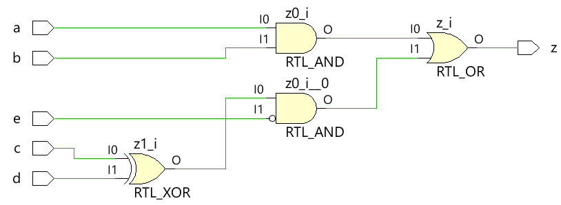
O código mostrado abaixo implementa uma lógica combinacional digital simples que possui um sinal de saída chamado z do tipo
reg que é atualizado sempre que um dos sinais na lista de sensibilidade altera seu valor. A lista de sensibilidade é declarada entre parênteses após o @ operador.
module combo ( 	input 	a, b, c, d, e,
								output 	reg z);

	always @ ( a or b or c or d or e) begin
		z = ((a & b) | (c ^ d) & ~e);
	end

endmodule
O módulo combo é elaborado no seguinte esquema de hardware usando ferramentas de síntese e pode ser visto que a lógica combinacional é implementada com portas digitais.
 Use atribuições de bloqueio ao modelar lógica combinacional com um bloco sempre
 Banco de teste
O testbench é uma plataforma para simular o projeto para garantir que o projeto se comporte conforme o esperado. Todas as combinações de entradas são direcionadas ao módulo de design usando um
for loop com uma declaração de atraso de 10 unidades de tempo para que o novo valor seja aplicado às entradas após algum tempo.
module tb;
	// Declare testbench variables
  reg a, b, c, d, e;
  wire z;
  integer i;

  // Instantiate the design and connect design inputs/outputs with
  // testbench variables
  combo u0 ( .a(a), .b(b), .c(c), .d(d), .e(e), .z(z));

  initial begin
  	// At the beginning of time, initialize all inputs of the design
  	// to a known value, in this case we have chosen it to be 0.
    a <= 0;
    b <= 0;
    c <= 0;
    d <= 0;
    e <= 0;

    // Use a $monitor task to print any change in the signal to
    // simulation console
    $monitor ("a=%0b b=%0b c=%0b d=%0b e=%0b z=%0b",
              a, b, c, d, e, z);

    // Because there are 5 inputs, there can be 32 different input combinations
    // So use an iterator "i" to increment from 0 to 32 and assign the value
    // to testbench variables so that it drives the design inputs
    for (i = 0; i < 32; i = i + 1) begin
      {a, b, c, d, e} = i;
      #10;
    end
  end
endmodule
Registro de simulação ncsim> run a=0 b=0 c=0 d=0 e=0 z=0 a=0 b=0 c=0 d=0 e=1 z=0 a=0 b=0 c=0 d=1 e=0 z=1 a=0 b=0 c=0 d=1 e=1 z=0 a=0 b=0 c=1 d=0 e=0 z=1 a=0 b=0 c=1 d=0 e=1 z=0 a=0 b=0 c=1 d=1 e=0 z=0 a=0 b=0 c=1 d=1 e=1 z=0 a=0 b=1 c=0 d=0 e=0 z=0 a=0 b=1 c=0 d=0 e=1 z=0 a=0 b=1 c=0 d=1 e=0 z=1 a=0 b=1 c=0 d=1 e=1 z=0 a=0 b=1 c=1 d=0 e=0 z=1 a=0 b=1 c=1 d=0 e=1 z=0 a=0 b=1 c=1 d=1 e=0 z=0 a=0 b=1 c=1 d=1 e=1 z=0 a=1 b=0 c=0 d=0 e=0 z=0 a=1 b=0 c=0 d=0 e=1 z=0 a=1 b=0 c=0 d=1 e=0 z=1 a=1 b=0 c=0 d=1 e=1 z=0 a=1 b=0 c=1 d=0 e=0 z=1 a=1 b=0 c=1 d=0 e=1 z=0 a=1 b=0 c=1 d=1 e=0 z=0 a=1 b=0 c=1 d=1 e=1 z=0 a=1 b=1 c=0 d=0 e=0 z=1 a=1 b=1 c=0 d=0 e=1 z=1 a=1 b=1 c=0 d=1 e=0 z=1 a=1 b=1 c=0 d=1 e=1 z=1 a=1 b=1 c=1 d=0 e=0 z=1 a=1 b=1 c=1 d=0 e=1 z=1 a=1 b=1 c=1 d=1 e=0 z=1 a=1 b=1 c=1 d=1 e=1 z=1 ncsim: *W,RNQUIE: Simulation is complete.
Observe que ambos os métodos,
assign e always , sejam implementados na mesma lógica de hardware. Exemplo nº 2:meio somador
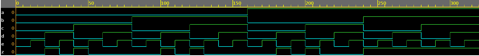
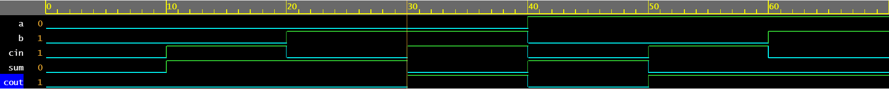
O módulo meio somador aceita duas entradas escalares aeb e usa lógica combinacional para atribuir a soma dos sinais de saída e o bit de transporte cout. A soma é acionada por um XOR entre a e b enquanto o bit de transporte é obtido por um AND entre as duas entradas.
module ha ( input 	a, b,
						output	sum, cout);

	always @ (a or b) begin
		{cout, sum} = a + b;
	end

endmodule
Banco de teste
module tb;
	// Declare testbench variables
  reg a, b;
  wire sum, cout;
  integer i;

  // Instantiate the design and connect design inputs/outputs with
  // testbench variables
  ha u0 ( .a(a), .b(b), .sum(sum), .cout(cout));

  initial begin
  	// At the beginning of time, initialize all inputs of the design
  	// to a known value, in this case we have chosen it to be 0.
    a <= 0;
    b <= 0;

    // Use a $monitor task to print any change in the signal to
    // simulation console
    $monitor("a=%0b b=%0b sum=%0b cout=%0b", a, b, sum, cout);

    // Because there are only 2 inputs, there can be 4 different input combinations
    // So use an iterator "i" to increment from 0 to 4 and assign the value
    // to testbench variables so that it drives the design inputs
    for (i = 0; i < 4; i = i + 1) begin
      {a, b} = i;
      #10;
    end
  end
endmodule
Registro de simulação ncsim> run a=0 b=0 sum=0 cout=0 a=0 b=1 sum=1 cout=0 a=1 b=0 sum=1 cout=0 a=1 b=1 sum=0 cout=1 ncsim: *W,RNQUIE: Simulation is complete.

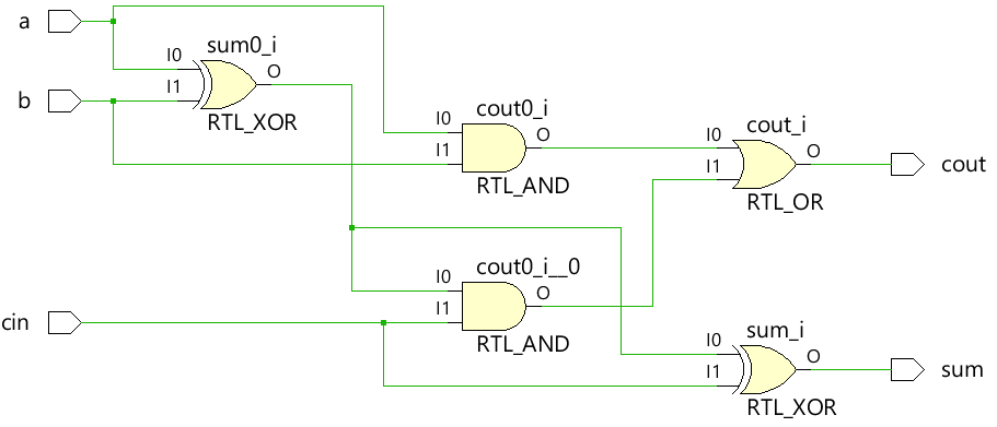
Exemplo nº 3:Somador Completo
Um bloco sempre pode ser usado para descrever o comportamento de um somador completo para direcionar a soma e o cout das saídas.
module fa (	input 	a, b, cin,
			output reg	sum, cout);

  always @ (a or b or cin) begin
    {cout, sum} = a + b + cin;
  end

endmodule
Banco de teste
module tb;
  reg a, b, cin;
  wire sum, cout;
  integer i;

  fa u0 ( .a(a), .b(b), .cin(cin), .sum(sum), .cout(cout));

  initial begin
    a <= 0;
    b <= 0;

    $monitor("a=%0b b=%0b cin=%0b cout=%0b sum=%0b", a, b, cin, cout, sum);

    for (i = 0; i < 8; i = i + 1) begin
      {a, b, cin} = i;
      #10;
    end
  end
endmodule
Registro de simulação ncsim> run a=0 b=0 cin=0 cout=0 sum=0 a=0 b=0 cin=1 cout=0 sum=1 a=0 b=1 cin=0 cout=0 sum=1 a=0 b=1 cin=1 cout=1 sum=0 a=1 b=0 cin=0 cout=0 sum=1 a=1 b=0 cin=1 cout=1 sum=0 a=1 b=1 cin=0 cout=1 sum=0 a=1 b=1 cin=1 cout=1 sum=1 ncsim: *W,RNQUIE: Simulation is complete.
Exemplo nº 4:Multiplexador 2x1
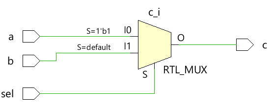
O multiplexador 2x1 simples usa um operador ternário para decidir qual entrada deve ser atribuída à saída c. Se sel for 1, a saída será acionada por a e se sel for 0, a saída será acionada por b.
module mux_2x1 (input 	a, b, sel,
				output 	reg c);


  always @ ( a or b or sel) begin
	c = sel ? a : b;
  end
endmodule
Banco de teste
module tb;
	// Declare testbench variables
  reg a, b, sel;
  wire c;
  integer i;

  // Instantiate the design and connect design inputs/outputs with
  // testbench variables
  mux_2x1 u0 ( .a(a), .b(b), .sel(sel), .c(c));

  initial begin
  	// At the beginning of time, initialize all inputs of the design
  	// to a known value, in this case we have chosen it to be 0.
    a <= 0;
    b <= 0;
    sel <= 0;

    $monitor("a=%0b b=%0b sel=%0b c=%0b", a, b, sel, c);

    for (i = 0; i < 3; i = i + 1) begin
      {a, b, sel} = i;
      #10;
    end
  end
endmodule
Registro de simulação ncsim> run a=0 b=0 sel=0 c=0 a=0 b=0 sel=1 c=0 a=0 b=1 sel=0 c=1 ncsim: *W,RNQUIE: Simulation is complete.

Exemplo nº 5:desmultiplexador 1x4
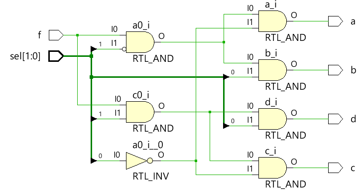
O demultiplexador usa uma combinação de entradas sel e f para acionar os diferentes sinais de saída. Cada sinal de saída é do tipo
reg e usado dentro de um always bloco que é atualizado com base nas alterações nos sinais listados na lista de sensibilidade.
module demux_1x4 (	input 				f,
										input [1:0]	 	sel,
										output reg		a, b, c, d);

  always @ ( f or sel) begin
    a = f & ~sel[1] & ~sel[0];
    b = f &  sel[1] & ~sel[0];
    c = f & ~sel[1] &  sel[0];
    d = f &  sel[1] &  sel[0];
  end

endmodule
Banco de teste
module tb;
	// Declare testbench variables
  reg f;
  reg [1:0] sel;
  wire a, b, c, d;
  integer i;

  // Instantiate the design and connect design inputs/outputs with
  // testbench variables
  demux_1x4 u0 ( .f(f), .sel(sel), .a(a), .b(b), .c(c), .d(d));

  // At the beginning of time, initialize all inputs of the design
  // to a known value, in this case we have chosen it to be 0.
  initial begin
    f <= 0;
    sel <= 0;

    $monitor("f=%0b sel=%0b a=%0b b=%0b c=%0b d=%0b", f, sel, a, b, c, d);

    // Because there are 3 inputs, there can be 8 different input combinations
    // So use an iterator "i" to increment from 0 to 8 and assign the value
    // to testbench variables so that it drives the design inputs
    for (i = 0; i < 8; i = i + 1) begin
      {f, sel} = i;
      #10;
    end
  end
endmodule
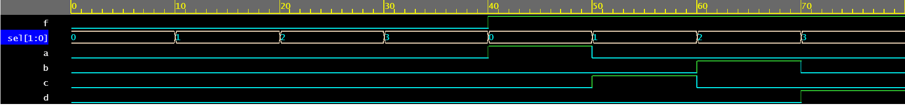
Registro de simulação ncsim> run f=0 sel=0 a=0 b=0 c=0 d=0 f=0 sel=1 a=0 b=0 c=0 d=0 f=0 sel=10 a=0 b=0 c=0 d=0 f=0 sel=11 a=0 b=0 c=0 d=0 f=1 sel=0 a=1 b=0 c=0 d=0 f=1 sel=1 a=0 b=0 c=1 d=0 f=1 sel=10 a=0 b=1 c=0 d=0 f=1 sel=11 a=0 b=0 c=0 d=1 ncsim: *W,RNQUIE: Simulation is complete.
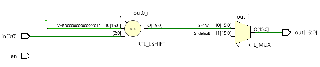
Exemplo nº 6:decodificador 4x16
module dec_3x8 ( 	input 			en,
					input 	[3:0] 	in,
					output  reg [15:0] 	out);

  always @ (en or in) begin
    out = en ? 1 << in: 0;
  end

endmodule
Banco de teste
module tb;
  reg en;
  reg [3:0] in;
  wire [15:0] out;
  integer i;

  dec_3x8 u0 ( .en(en), .in(in), .out(out));

  initial begin
    en <= 0;
    in <= 0;

    $monitor("en=%0b in=0x%0h out=0x%0h", en, in, out);

    for (i = 0; i < 32; i = i + 1) begin
      {en, in} = i;
      #10;
    end
  end
endmodule
Registro de simulação ncsim> run en=0 in=0x0 out=0x0 en=0 in=0x1 out=0x0 en=0 in=0x2 out=0x0 en=0 in=0x3 out=0x0 en=0 in=0x4 out=0x0 en=0 in=0x5 out=0x0 en=0 in=0x6 out=0x0 en=0 in=0x7 out=0x0 en=0 in=0x8 out=0x0 en=0 in=0x9 out=0x0 en=0 in=0xa out=0x0 en=0 in=0xb out=0x0 en=0 in=0xc out=0x0 en=0 in=0xd out=0x0 en=0 in=0xe out=0x0 en=0 in=0xf out=0x0 en=1 in=0x0 out=0x1 en=1 in=0x1 out=0x2 en=1 in=0x2 out=0x4 en=1 in=0x3 out=0x8 en=1 in=0x4 out=0x10 en=1 in=0x5 out=0x20 en=1 in=0x6 out=0x40 en=1 in=0x7 out=0x80 en=1 in=0x8 out=0x100 en=1 in=0x9 out=0x200 en=1 in=0xa out=0x400 en=1 in=0xb out=0x800 en=1 in=0xc out=0x1000 en=1 in=0xd out=0x2000 en=1 in=0xe out=0x4000 en=1 in=0xf out=0x8000 ncsim: *W,RNQUIE: Simulation is complete.

Verilog
- Tutorial - Escrevendo Código Combinacional e Sequencial
- Circuito com interruptor
- Circuitos integrados
- Introdução à Álgebra Booleana
- Aritmética com notação científica
- Perguntas e respostas com um arquiteto de soluções da indústria 4.0
- Monitorando a temperatura com Raspberry Pi
- Exemplos de nível de portão Verilog
- Formato de hora Verilog
- Sempre um acabamento suave com as retificadoras Okamoto