


Nanohelix de porta dupla como uma nova superrede binária ajustável
Resumo
Teoricamente, investigamos o problema de um elétron confinado a uma nanohélice entre duas portas paralelas modeladas como fios carregados. O sistema nanohelix de dupla passagem é uma superrede binária com propriedades altamente sensíveis às tensões da porta. Em particular, a estrutura de banda exibe cruzamentos de banda de energia para certas combinações de tensões de porta, o que poderia levar a fenômenos quase relativísticos do tipo Dirac. Nossa análise para transições ópticas induzidas por luz polarizada linear e circularmente sugere que uma nanohélice de dupla entrada pode ser usada para aplicações optoeletrônicas versáteis.
Introdução
Dos gastrópodes fossilizados em espiral que o primeiro autor coletou com entusiasmo em sua infância, à estrutura entrelaçada do DNA que, sem dúvida, uma vez definiu essas criaturas pré-históricas, a geometria da hélice prevalece em toda a natureza [1]. Inspirado nas funcionalidades complexas atribuídas às formas de biomoléculas de ocorrência natural [2–6], espera-se que outros sistemas possuindo geometrias helicoidais adequadas para nanotecnologia gerem física rica e contribuam para novas aplicações. Nas últimas três décadas, o progresso notável em técnicas de nanofabricação levou à realização de nanohelices em uma série de sistemas diferentes, incluindo InGaAs / GaAs [7], Si / SiGe [8], ZnO [9-11], CdS [ 12], SiO 2 / SiC [13, 14], e carbono puro [15–20], bem como semicondutores II-VI e III-V [21] (para o estado atual da arte, consulte as Refs. [21–26]). Consequentemente, uma infinidade de fenômenos é esperada em tais estruturas que variam de propriedades de transporte exóticas, como bombeamento de carga quantizada topológica [27, 28], supercondutividade [29] e filtragem de spin [30-32], à eletrônica extensível molecular e nanomecânica [33, 34] devido a efeitos piezoelétricos [35], aplicações de detecção [36, 37], armazenamento de energia [38] e hidrogênio [39] e transistores de efeito de campo [40, 41].
O fascínio pelos dispositivos baseados em nanohélice, em última análise, origina-se da periodicidade inerente codificada na topologia da estrutura da hélice. Em particular, submeter uma nanohélice a um campo elétrico transversal (normal ao eixo da hélice) dá origem a um comportamento de superrede, como o espalhamento de elétrons de Bragg em um potencial superperiódico, levando a uma divisão de energia na borda da zona de Brillouin de superrede entre os estados mais baixos linearmente ajustáveis pelo campo elétrico [42, 43]. Este comportamento pode resultar em oscilações de Bloch e condutância diferencial negativa [44, 45], e pode enfatizar o transporte polarizado por spin através de hélices [31, 46], bem como produzir um aumento de dicroísmo circular útil em aplicações quirópticas nanofotônicas [47]. Este sistema constitui uma superrede unária e ainda abre a possibilidade de usar nanohelices como díodos túnel ou díodos Gunn para multiplicação de frequência, amplificação e geração ou absorção de radiação na faixa terahertz eulogizada [48-51]. Enquanto a superrede prototípica é geralmente realizada em heteroestruturas de camadas semicondutoras alternadas com diferentes intervalos de banda intrínsecos, os parâmetros da superrede nanohelix são totalmente controlados pelo campo externo. Contrariamente, as formas dos antigos potenciais de superrede convencionais são específicas para a heteroestrutura e, embora robustas, oferecem capacidade limitada de manipulação no curso de sua exploração sem o uso de grandes campos externos. Portanto, o apelo em usar nanohelices como superredes em vez disso está em sua maior sintonia.
Por outro lado, com superredes semicondutoras de heteroestrutura (ou mesmo estruturas de superrede fotônica [52-55] e átomos frios em redes ópticas [56, 57]), pode-se criar células unitárias de superrede mais complicadas além do poço quântico simples que é induzido pelo campo elétrico ao longo da hélice. Até mesmo a extensão para uma superrede binária [58-60] (em que a célula unitária é distinguida por dois poços quânticos diferentes e / ou barreiras) promete uma rica gama de física, como oscilações Bloch-Zener [61], que por sua vez pode contribuir para aplicações de divisor de feixe e interferômetro sintonizáveis [62]. Assim, seria altamente desejável combinar a sintonia de campo externo de uma superrede baseada em nanohelix com a funcionalidade superior de uma superrede binária.
A seguir, descrevemos esse sistema, com uma nanohélice posicionada entre dois fios carregados com portas paralelas alinhadas com o eixo da hélice. Prevemos a aplicação de um campo elétrico transversal adicional e, teoricamente, mostrar que o potencial controlável de porta e campo constitui uma superrede binária ao longo da hélice unidimensional.
Métodos
Modelo teórico
Vamos começar estudando o caso de uma nanohélice circular semicondutora de elétron único com N voltas do raio R , pitch p , e comprimento total L = Np . A nanoestrutura é posicionada entre duas portas paralelas modeladas como fios carregados com seu eixo de hélice alinhado ao longo do z -eixo e com eixo e portas todos residindo no mesmo plano, conforme ilustrado na Fig. 1. Além disso, consideramos um campo elétrico transversal externo normal ao plano do eixo da porta \ (\ mathbf {E} =E _ {\ bot} \ hat {\ mathbf {y}} \) que pode ser usado para quebrar a simetria de reflexão do potencial acima do plano em relação ao potencial abaixo do plano. Trabalhamos em coordenadas helicoidais descritas parametricamente via r =( x, y , z ) =( R cos ( s φ ), R pecado ( s φ ), ρ φ ), onde a coordenada angular dinâmica φ = z / ρ depende apenas da distância ao longo do eixo da hélice com ρ = p / 2 π e s =± 1 indica uma hélice esquerda ou direita, respectivamente. Neste trabalho, consideramos uma hélice canhota s =1. Na estrutura do modelo de massa efetiva, o espectro de energia ε ν do ν o autoestado de um elétron em uma hélice sob a influência de tais potenciais externos é encontrado a partir da equação de Schrödinger:
$$ - \ thinspace \ frac {\ hbar ^ {2}} {2M ^ {*} \ rho ^ {2}} \ frac {d ^ {2}} {d \ varphi ^ {2}} \ psi _ {\ nu} + \ left [V_ {g} (\ varphi) + V _ {\ bot} (\ varphi) \ right] \ psi _ {\ nu} =\ varejpsilon _ {\ nu} \ psi _ {\ nu} $$ (1 )
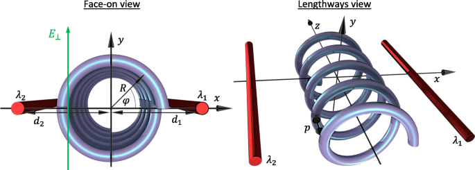
Diagrama da geometria e parâmetros do sistema de ambas as perspectivas de face e longitudinal. R é o raio da hélice e d 1 e d 2 são as distâncias dos fios carregados do eixo da hélice com densidades de carga λ 1 e λ 2 , respectivamente. A coordenada espacial φ descreve a posição angular na hélice de frente e está relacionada ao z -coordenar via φ =2 π z / p com p o passo da hélice. Um campo elétrico transversal E ⊥ é aplicado paralelamente ao y -eixo
onde renormalizamos geometricamente a massa efetiva do elétron M e para M ∗ = M e (1+ R 2 / ρ 2 ) para expressar tudo em termos de coordenadas ao longo do eixo da hélice (lembre-se de que φ = z / ρ ) que é mais conveniente para potenciais externos. Aqui, V ⊥ ( φ ) =- eE ⊥ R pecado ( φ ) é a contribuição do campo elétrico transversal direcionado ao longo do y -eixo tal que V ⊥ ( π / 2) <0. O potencial dos portões é V g ( φ ) =- e [ Φ 1 ( φ ) + Φ 2 ( φ )] com o potencial eletrostático sentido por um elétron ao longo da hélice devido a um fio individual carregado dado por Φ i ( φ ) =- λ i k ln ( r i / d i ) Aqui, i =1,2 rotula os fios, λ i é a densidade de carga linear em um fio e \ (k =1/2 \ pi \ tilde {\ epsilon} \) com \ (\ tilde {\ epsilon} \) a permissividade absoluta. A distância perpendicular de uma carga de teste de um fio específico é dada por \ (r_ {i} =[d ^ {2} _ {i} + R ^ {2} + 2 (-1) ^ {i} d_ {i } R \ cos (\ varphi)] ^ {1/2} \), com d i denotando a distância correspondente do fio ao eixo da hélice. Definimos o potencial induzido pela porta zero ao longo do eixo da hélice. O potencial unidimensional total V T ( φ ) = V g ( φ ) + V ⊥ ( φ ) é claramente periódico V T ( φ ) = V T ( φ +2 π n ) com período 2 π em geral (que corresponde ao período de p em relação à coordenada z ) Este período é significativamente maior do que a distância interatômica e dá origem a efeitos de superrede típicos. Esta letra difere de uma nanohélice em um campo elétrico transversal (que pode ser reproduzido com V T ( φ ) = V ⊥ ( φ ) aqui) principalmente manipulando a célula unitária repetida da superrede por meio do potencial de porta dupla V g ( φ ) Tomando o limite p → 0, voltamos à partícula em uma imagem do anel sujeita a duas portas eletrostáticas [63, 64]. Fazendo a aproximação R / d i ≪1, podemos expandir V g ( φ ) até a segunda ordem em cos ( φ ), e ao transformar a Eq. 1 na forma adimensional, chegamos a
$$ {\ begin {alinhados} \ frac {d ^ {2} \ psi _ {\ nu}} {d \ varphi ^ {2}} + \ left [\ epsilon _ {\ nu} + 2A_ {g} \ cos ( \ varphi) + 2B_ {g} \ cos (2 \ varphi) + 2C _ {\ bot} \ sin (\ varphi) \ right] \ psi _ {\ nu} =0, \ end {alinhado}} $$ (2)
com as quantidades em unidades da escala de energia \ (\ varepsilon _ {0} (\ rho) =\ hbar ^ {2} / 2 M ^ {*} \ rho ^ {2} \) definido como
$$ \ begin {array} {@ {} rcl @ {}} A_ {g} &=&\ beta \ frac {\ left (d_ {1} ^ {2} + R ^ {2} \ right)} { d_ {1} R} (1- \ gamma), \ qquad B_ {g} =\ frac {\ beta} {2} \ left (1+ \ frac {\ lambda_ {1}} {\ lambda_ {2}} \ gamma ^ {2} \ right), \\ C _ {\ bot} &=&e E _ {\ bot} R / 2 \ varepsilon_ {0} (\ rho), \ qquad \ qquad \ qquad \; \ epsilon _ {\ nu} =\ frac {\ varepsilon _ {\ nu}} {\ varepsilon_ {0} (\ rho)}. \ end {array} $$ (3)
Aqui, \ (\ beta =ek d_ {1} ^ {2} R ^ {2} \ lambda _ {1} / 2 \ left (d_ {1} ^ {2} + R ^ {2} \ right) ^ {2} \ varepsilon _ {0} (\ rho) \) caracteriza a contribuição do portão 1 enquanto o parâmetro de assimetria \ (\ gamma =\ lambda _ {2} d_ {2} \ left (d_ {1} ^ {2 } + R ^ {2} \ right) / \ lambda _ {1} d_ {1} \ left (d_ {2} ^ {2} + R ^ {2} \ right) \) caracteriza a contribuição relativa do portão 2 , com γ =1 correspondendo a contribuições de portão iguais para o potencial (resultando em A g =0). Deve-se notar que a inevitável assimetria causada pela dificuldade em manter d 1 = d 2 pode ser compensado pela manipulação de λ 1 e λ 2 . Nesta carta, nos restringimos a considerar γ ≤1 (que é | Φ 1 |> | Φ 2 |) como o parâmetro de assimetria sendo maior que a unidade pode ser mapeado para um sistema equivalente abaixo da unidade por meio de uma simples troca dos índices que rotulam as portas e a mudança de perspectiva correspondente φ → φ ± π . Também consideraremos apenas C ⊥ ≥0 devido à simetria de C negativa ⊥ com relação a tal tradução de coordenadas em φ e A g ≥0, B g > 0 (ou seja, apenas densidades de carga positiva nos fios β > 0) pois qualquer paisagem potencial com portas carregadas negativamente pode ser reproduzida com a combinação correta de parâmetros de portas carregadas positivamente. Na Fig. 2, traçamos o potencial adimensional V T ( φ ) / ε 0 ( ρ ), com a força do π - componente potencial periódico fixado em B g =0,2, para várias combinações dos parâmetros de perturbação de período dobrado A g e C ⊥ . Vemos que o potencial externo total induz uma superrede binária ao longo de φ , com um poço quântico duplo (DQW) como uma célula unitária destacada em azul. Isso pode assumir formas qualitativamente diferentes, manipulando as contribuições relativas da porta γ e campo elétrico transversal E ⊥ . A célula unitária é essencialmente um único poço sob contribuições de porta equivalentes ( γ =1) e nenhum campo elétrico transversal E ⊥ =0 (como na Fig. 2a para A g = C ⊥ =0). Consertando E ⊥ =0, com uma contribuição de portão 1 mais forte ( γ <1), a célula unitária torna-se um DQW com diferentes bem mínimos e máximos de barreira degenerada (Fig. 2b onde A g =0.1 e C ⊥ =0). Em contraste, manter os mínimos DQW degenerados e manipular as duas barreiras potenciais em relação uma à outra requer contribuições de porta simétrica ( γ =1) em um campo elétrico diferente de zero E ⊥ ≠ 0 (Fig. 2c com A g =0 e C ⊥ =0,1). Combinando contribuições de porta assimétrica ( γ <1) com E ⊥ ≠ 0 produz um DQW com diferentes potenciais mínimos do poço e diferentes barreiras (como visto na Fig. 2d onde ambos A g = C ⊥ =0,1). Isso leva a um comportamento qualitativamente diferente e rico, como veremos nas próximas seções.
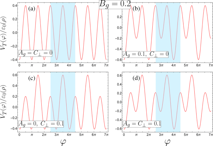
As quatro configurações de potencial de superrede possíveis com as células unitárias destacadas em azul (definidas em termos de parâmetros adimensionais, consulte a Eq. 3 para os requisitos correspondentes dos parâmetros físicos, e todas com B g =0,2). a Uma superrede unária com mínimos e máximos degenerados na célula unitária ( A g = C ⊥ =0). b - d Superredes binárias formadas de b um DQW assimétrico com mínimos diferentes e simetria de reflexão interna sobre os mínimos devido a máximos degenerados ( A g =0,1, C ⊥ =0), c um DQW simétrico com mínimos degenerados apenas ( A g =0, C ⊥ =0,1), ou d um DQW assimétrico com mínimos e máximos diferentes ( A g = C ⊥ =0,1)
Soluções como uma matriz infinita
Soluções para a Eq. 2 pode ser encontrado em termos das funções de Bloch
$$ \ psi_ {n, q} (\ varphi) =(2 \ pi N \ rho) ^ {- \ frac {1} {2}} e ^ {iq \ varphi} \ sum_ {m} c ^ {( n)} _ {m, q} e ^ {im \ varphi}, $$ (4)
onde o q = k z ρ é a forma adimensional do quasimomentum do elétron k z ao longo do eixo da hélice, n indica a sub-banda, e o prefator surge da normalização em termos de φ :\ (\ rho \ int _ {0} ^ {2 \ pi N} | \ psi _ {n, q} (\ varphi) | ^ {2} d \ varphi =1 \). Fazemos uso da ortogonalidade das funções exponenciais multiplicando a expressão resultante por \ (e ^ {im ^ {\ prime} \ varphi} / 2 \ pi \) e integrando em relação a φ , onde m ′ é um número inteiro, de modo que chegamos a um conjunto infinito de equações simultâneas para os coeficientes \ (c ^ {(n)} _ {m, q} \),
$$ {\ begin {alinhados} &\ left [(q + m) ^ {2} - \ epsilon_ {n} \ right] c ^ {(n)} _ {m} - \ left (A_ {g} - i C _ {\ bot} \ right) c ^ {(n)} _ {m-1} - \ left (A_ {g} + i C _ {\ bot} \ right) c ^ {(n)} _ {m +1} \\ &\ quad- B_ {g} \ left (c ^ {(n)} _ {m + 2} + c ^ {(n)} _ {m-2} \ right) =0, \ fim {alinhado}} $$ (5)
onde, para maior clareza, o q -a notação de subscrito foi eliminada, ε n, q ≡ ε n e \ (c_ {m} ^ {(n)} \ equiv c_ {m, q} ^ {(n)} \). A Equação 5 representa uma matriz penta-diagonal infinita em que é aparente que o sistema é periódico em q , e podemos restringir nossas considerações à primeira zona de Brillouin definida por - 1 / 2≤ q ≤1 / 2. Na ausência do potencial de superrede A g = B g = C ⊥ =0, os valores próprios são enumerados por m fornecido por ε m =( m + q ) 2 e reconhecemos m ser o número quântico do momento angular associado a um elétron livre em uma hélice. Vemos na Eq. 5 que quando A g = C ⊥ =0 apenas estados com Δ m =± 2 são misturados, enquanto a formação de uma célula unitária DQW com diferentes mínimos de poço ou barreiras, alcançada por meio de A g ≠ 0 e / ou C ⊥ ≠ 0, também mistura estados com Δ m =± 1. Curiosamente, o sistema de um elétron em uma hélice sob um potencial transversal externo (que varia ao longo de uma revolução da hélice) é matematicamente equivalente a um elétron em um anel quântico perfurado por um campo magnético e sujeito a um potencial com a mesma forma funcional variando ao longo da coordenada angular; por exemplo. ver Ref. [65–67] ou compare, por exemplo, as Refs. [42–45] com [68–70]. Para um anel, o papel desempenhado por q aqui é absorvido pelo fluxo magnético. Conseqüentemente, exatamente a mesma análise neste trabalho é aplicável ao problema de um anel quântico de dupla passagem [63-66], onde o anel é perfurado por um fluxo magnético.
Truncando e diagonalizando numericamente a matriz correspondente à Eq. 5 fornece o n autoenergias de sub-banda ε n e coeficientes \ (c_ {m} ^ {(n)} \) para cada valor de q . Aplicamos um truncamento em | m | =10, com a certeza de que qualquer aumento no tamanho da matriz não produz nenhuma mudança apreciável nas sub-bandas mais baixas.
Resultados e discussão
Estrutura de banda de nanohelix de porta dupla
Representamos graficamente na Fig. 3 a dispersão de energia das bandas mais baixas para várias combinações de parâmetros. Dependendo da forma da superrede, encontramos uma variedade notável no comportamento de dispersão e, para algumas combinações específicas de parâmetros, descobrimos cruzamentos de bandas de energia para sub-bandas particulares na borda da zona de Brillouin (Fig. 3a e c) ou no centro da zona de Brillouin (Fig. 3b e d).
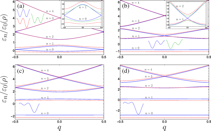
Estrutura de banda para o sistema nanohelix de duplo portão para várias combinações dos parâmetros adimensionais (com B g =0,4 fixo em toda): a Plotagens em azul sólido (vermelho tracejada) A g =0 e C ⊥ =0 ( A g =0,2 & C ⊥ =0), a inserção representa adicionalmente o comportamento das duas sub-bandas inferiores sujeitas ao campo elétrico transversal com A g =0 e C ⊥ =0,2 como a curva verde pontilhada e tracejada. b Plotagens em azul sólido (vermelho tracejada) A g =0,63 & C ⊥ =0 ( A g =0,8 & C ⊥ =0) onde a curva azul representa o primeiro incidente de ressonância (ver texto) com bandas de energia cruzando no centro da zona de Brillouin, a inserção compara o comportamento das duas sub-bandas excitadas de baixo com o caso em que A g =0,63 & C ⊥ =0,2 como a curva verde pontilhada e tracejada. c Plotagens em azul sólido (vermelho tracejada) A g =1,26 & C ⊥ =0 ( A g =1,5 & C ⊥ =0) onde a curva azul representa o segundo incidente de ressonância com lacunas de energia fechando na borda do Brillouin para bandas mais altas. d A terceira ressonância e os minigaps de sub-banda superiores fecham no centro, com o azul sólido (vermelho tracejada) sendo A g =1.9 & C ⊥ =0 ( A g =2.2 & C ⊥ =0). As formas das células unitárias são esboçadas, n enumera as bandas, e os eixos das inserções são os mesmos dos gráficos principais
Perturbação de período dobrado de campo baixo
Quando A g = C ⊥ =0, a célula unitária constitui dois poços quânticos equivalentes e, conseqüentemente, o aparecimento de pares de bandas tocando nas bordas da zona de Brillouin surge naturalmente. Na verdade, tomar apenas um poço como a célula unitária reduz pela metade o período da superrede e resulta em uma duplicação da zona de Brillouin - 1≤ q ≤1. Em seguida, observaríamos o diagrama de bandas de superrede unário usual, em que o gap entre o solo e as primeiras bandas em q =1 é dado aqui através do gap entre n =1 e n =2 em q =0 e seria linear em B g da teoria da perturbação. Ainda assim, apresentamos uma descrição da estrutura da banda em | q | =1/2 na imagem de célula unitária DQW usando álgebra matricial no apêndice. Como visto na inserção da Fig. 3a, a introdução de qualquer um dos termos de potencial de período duplo abre um gap na borda da zona de Brillouin. A célula unitária das contribuições de porta simétrica ( A g =0) retém a forma de um DQW simétrico sob a aplicação de um campo transversal C ⊥ perpendicular ao eixo helix-gate, com uma barreira potencial modificada em relação à outra (indicada pelo esboço DQW verde na Fig. 3a). Enquanto C ⊥ abre uma lacuna de banda, a modificação da dispersão é notavelmente menos sensível do que aquela de uma magnitude semelhante de A aplicada g . Isso é visto pelo menor intervalo de banda em | q | =1/2 para a linha verde pontilhada e tracejada na inserção da Fig. 3a (com A g =0 e C ⊥ =0,2) em comparação com a lacuna maior para a curva vermelha tracejada (que é para A g =0,2 e C ⊥ =0). Para enfatizar este comportamento, a Fig. 4a plota o tamanho do gap de energia em | q | =1/2 entre as duas sub-bandas mais baixas \ (\ Delta \ varepsilon _ {01} ^ {(q =1/2)} / \ varepsilon _ {0} (\ rho) \) para B g =0,25 em função de ambos C ⊥ (com A g =0) e A g (com C ⊥ =0), como curvas pontilhadas verdes e vermelhas tracejadas, respectivamente. Em campo elétrico transversal zero e potenciais de porta assimétrica ( C ⊥ =0 e A g ≠ 0), a célula unitária é então um DQW assimétrico, embora com simetria de reflexão interna sobre os mínimos do poço devido às barreiras equivalentes. Podemos, então, compreender a maior sensibilidade do intervalo de banda à alteração de A g considerando as propriedades da célula unitária DQW isolada a partir da qual a superrede é construída. Com A g = C ⊥ =0, em | q | =1/2 (as bordas da zona de Brillouin), os estados de Bloch formados a partir do solo e primeiro estado excitado da célula unitária DQW isolada (ver o esquema azul e as funções de onda acompanhantes na Fig. 4a) irão diferir apenas por um fase arbitrária. Esta situação corresponde à curva de dispersão azul sem intervalos da Fig. 3a. Conforme representado esquematicamente na Fig. 4a através do esboço DQW verde, C ⊥ reduz os máximos relativos de uma das barreiras em relação à outra, enquanto os mínimos DQW permanecem degenerados. Como tal, o estado fundamental do DQW isolado é modificado apenas por um ligeiro aumento na sua distribuição de probabilidade sob a barreira de potencial menor (produzindo apenas uma pequena redução na energia em comparação com o estado fundamental não perturbado), e o primeiro estado excitado permanece essencialmente inalterado pois seu nó está posicionado sob a barreira e não é sensível à sua variação. Os estados de Bloch na borda da zona de Brillouin que são construídos a partir desses estados básicos e excitados diferem do caso não perturbado apenas no decaimento reduzido da função de onda do estado fundamental sob a barreira menor (compare o DQW verde com o DQW azul em Fig. 4a). Alterando A g manipula as posições relativas dos mínimos DQW enquanto mantém as barreiras degeneradas. As funções de onda dos dois estados DQW isolados mais baixos diferem consideravelmente, com o estado fundamental tendendo para o estado fundamental localizado do poço mais profundo singular e o primeiro estado excitado tendendo para o estado fundamental localizado do poço mais raso [71]. Enquanto a perturbação reduz a energia do estado fundamental, a energia do primeiro estado excitado é comparativamente aumentada conforme os mínimos do poço mais raso são deslocados para cima com o aumento de A g , resultando na maior sensibilidade do tamanho do gap em relação a A g . Em particular, uma partícula na sub-banda terrestre rapidamente se encontra confinada perto do fundo do poço de potencial mais profundo com o aumento de A g . A banda mais baixa, portanto, se aproxima de uma banda plana sem dispersão mais rápida do que no caso do campo transversal, o que pode levar a instabilidades eletrônicas e fortes efeitos de interação que acompanham a alta densidade de estados [72].
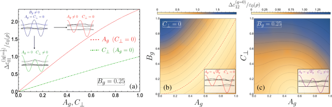
a Tamanho da lacuna de banda entre o solo e as primeiras sub-bandas em função de A g ( C ⊥ ) plotado como vermelho tracejada (verde tracejada), aqui B g =0,25. Os diagramas indicam a influência das diferentes perturbações na célula unitária DQW isolada e nos estados próprios. b - c Tamanho do intervalo de banda entre a primeira e a segunda sub-bandas indicado através de um gráfico de densidade 2D em função de; b A g e B g para C ⊥ =0 e c A g e C ⊥ com B fixo g =0,25. b As linhas de contorno de isoenergia adjacentes indicam uma diferença de 0,17, com intervalo zero dado pela linha vermelha pontilhada para \ (A_ {g} =\ sqrt {B_ {g}} \), enquanto c a diferença é 0,13 com lacuna zero no centro do contorno de semicírculo menor (0,5,0). Os diagramas esboçam o DQW e os estados próprios isolados. A hibridização não ocorre entre os s -como e p - como estados de poços individuais localizados ressonantes em b , mas faz em c devido ao campo elétrico mudando uma barreira em relação à outra
Cruzamentos de faixa de energia
É bastante notável ver que se mantivermos C ⊥ =0 e aumentar A g , embora inicialmente todas as degenerescências sejam levantadas, as bandas de energia superior subsequentes são trazidas para se cruzarem alternando entre o centro e a borda da zona de Brillouin (observe o comportamento das curvas azuis e vermelhas tracejadas alternadas progredindo da Fig. 3a até a d). Fisicamente, podemos entender a lacuna de banda que desaparece em termos de interações das funções de onda localizadas na célula unitária. Quando o potencial DQW assimétrico é tal que o estado fundamental no poço mais raso ( s -como orbital) é ressonante com o primeiro estado excitado no poço mais profundo ( p -como orbital), em q =0 devido à simetria de reflexão sobre o centro de cada poço, as paridades opostas desses estados impedem o acoplamento de túnel usual entre eles e, consequentemente, os estados excitados construídos a partir desses orbitais coincidem (curvas azuis na Fig. 3b). Isso é uma reminiscência dos chamados s - p ressonâncias em redes ópticas [73, 74]. Da mesma forma, se os parâmetros são tais que o estado fundamental localizado no poço raso é ressonante com um estado excitado no poço mais profundo tendo a mesma paridade, então em | q | =1/2, a presença da fase de Bloch suprime totalmente a hibridização usual entre esses dois estados de poço localizados adjacentes e o gap é fechado (como mostrado na Fig. 3c para ressonância do solo com o segundo estado excitado). Na linguagem da dispersão do potencial periódico; o gap é fechado devido à interferência destrutiva completa das amplitudes de espalhamento de Bragg de segunda ordem do cos ( φ ) potencial e amplitudes de espalhamento de primeira ordem do cos (2 φ ) potencial [75–77].
Podemos mostrar quantitativamente a existência de cruzamentos de banda de energia (para campo elétrico transversal zero) no centro e na borda da zona de Brillouin, retornando à Eq. 2, que é reconhecível como a equação de Whittaker-Hill quando C ⊥ =0 [78]. As funções de Bloch Eq. 4 obedecer às condições de contorno periódicas torcidas ψ n, q ( φ +2 π ) =exp (2 π iq ) ψ n, q ( φ ) Em particular, quando q =0 soluções formais para a Eq. 2 são 2 π -periódico, enquanto quando | q | =1/2 soluções são 2 π -antiperiódico (e, portanto, devemos pesquisar 4 π -soluções periódicas). Especificamente, a Eq. 2 com C ⊥ =0 pode ser mapeado para a equação de Ince [79, 80], que é quase exatamente resolvível, por meio da expressão da função de onda como o produto da solução assintótica para a Eq. 2 e uma função desconhecida \ (\ psi _ {n, q} (\ varphi) =\ exp \ left [-2 \ sqrt {B_ {g}} \ cos (\ varphi) \ right] \ Phi _ {n, q} (\ varphi) \), de modo que
$$ \ frac {d ^ {2} \ Phi_ {n, q}} {d \ varphi ^ {2}} + \ frac {\ xi} {2} \ sin (\ varphi) \ frac {d \ Phi_ { n, q}} {d \ varphi} + \ frac {1} {4} \ left [\ eta_ {n, q} - p \ xi \ cos (\ varphi) \ right] \ Phi_ {n, q} =0, $$ (6)
onde definimos os parâmetros auxiliares \ (\ xi =8 \ sqrt {B_ {g}} \), η n, q =4 ε n, q +8 B g , \ (- p \ xi =8A_ {g} +8 \ sqrt {B_ {g}} \), e Φ n, q ( φ ) mantém a periodicidade torcida necessária de cada solução (observe que aqui p é não o passo da hélice). Além disso, como o potencial de superrede aqui é invariante sob a transformação φ → - φ , as soluções para q =0 e q =1/2 pode ser separado em paridade ímpar e par, de modo que a seguinte série trigonométrica
$$ \ Phi_ {n, 0} ^ {(e)} (\ varphi) =\ sum_ {l =0} a ^ {(n)} _ {l} \ cos (l \ varphi), $$ (7a ) $$ \ Phi_ {n, 0} ^ {(o)} (\ varphi) =\ sum_ {l =0} b ^ {(n)} _ {l + 1} \ sin [(l + 1) \ varphi], $$ (7b) $$ \ Phi_ {n, \ frac {1} {2}} ^ {(e)} (\ varphi) =\ sum_ {l =0} \ widetilde {a} ^ {( n)} _ {l} \ cos \ left [\ left (l + \ frac {1} {2} \ right) \ varphi \ right], $$ (7c) $$ \ Phi_ {n, \ frac {1} {2}} ^ {(o)} (\ varphi) =\ sum_ {l =0} \ widetilde {b} ^ {(n)} _ {l + 1} \ sin \ left [\ left (l + \ frac {1} {2} \ right) \ varphi \ right], $$ (7d)
cobrem as soluções formais, e notamos que as soluções para q =−1 / 2 são iguais para q =1/2. Aqui, os sobrescritos e e o rotule as funções como pares e ímpares, respectivamente, e n ainda se refere ao n a sub-banda, que também é a n o autoestado para estes especificados q valores. Substituindo-os na Eq. 6 resulta em relações de recursão de três termos para os coeficientes de Fourier. O q =0 rendimento de solução par
$$ - \ eta_ {n, 0} ^ {(e)} a ^ {(n)} _ {0} + \ xi \ left (\ frac {p} {2} +1 \ right) a ^ {( n)} _ {2} =0, $$ (8a) $$ \ xi pa ^ {(n)} _ {0} + \ left (4 - \ eta_ {n, 0} ^ {(e)} \ direita) a ^ {(n)} _ {2} + \ xi \ left (\ frac {p} {2} +2 \ right) a ^ {(n)} _ {4} =0, $$ (8b ) $$ {\ begin {alinhados} &\ xi \ left (\ frac {p} {2} - l +1 \ right) a ^ {(n)} _ {2l-2} + \ left (4l ^ { 2} - \ eta_ {n, 0} ^ {(e)} \ right) a ^ {(n)} _ {2l} \\ &\ quad + \ xi \ left (\ frac {p} {2} + l +1 \ direita) a ^ {(n)} _ {2l + 2} =0, \ qquad (l \ ge 2) \ end {alinhado}} $$ (8c)
e as relações de recursão correspondentes para a solução ímpar para q =0 é
$$ (4 - \ eta_ {n, 0} ^ {(o)}) b ^ {(n)} _ {2} + \ xi \ left (\ frac {p} {2} +2 \ right) b ^ {(n)} _ {4} =0, $$ (9a) $$ {\ begin {alinhado} &\ xi \ left (\ frac {p} {2} - l +1 \ right) b ^ { (n)} _ {2l-2} + \ left (4l ^ {2} - \ eta_ {n, 0} ^ {(o)} \ right) b ^ {(n)} _ {2l} + \ xi \ left (\ frac {p} {2} + l +1 \ right) b ^ {(n)} _ {2l + 2} \\ &=0. \ qquad (l \ ge 2) \ end {alinhado} } $$ (9b)
O q =1/2 solução uniforme dá
$$ \ left [1 - \ eta_ {n, \ frac {1} {2}} ^ {(e)} + \ frac {\ xi} {2} (p + 1) \ right] \ widetilde {a} ^ {(n)} _ {1} + \ frac {\ xi} {2} (p + 3) \ widetilde {a} ^ {(n)} _ {3} =0, $$ (10a) $$ {}{\begin{aligned} &\frac{\xi}{2}(p-2l +1)\widetilde{a}^{(n)}_{2l-1}+\left[(2l+1 )^{2} - \eta_{n,\frac{1}{2}}^{(e)}\right]\widetilde{a}^{(n)}_{2l+1}\\ &\ quad+ \frac{\xi}{2}(p+2l+3)\widetilde{a}^{(n)}_{2l+3}=0, \qquad (l \ge 1) \end{aligned} } $$ (10b)
and the q =1/2 odd solution gives
$$ \left[ 1 -\eta_{n,\frac{1}{2}}^{(e)} -\frac{\xi}{2}(p+1) \right]\widetilde{b}^{(n)}_{1} +\frac{\xi}{2}(p+3)\widetilde{b}^{(n)}_{3}=0 $$ (11a) $$ {}{\begin{aligned} &\frac{\xi}{2}(p-2l+1)\widetilde{b}^{(n)}_{2l-1}+\left[(2l+1)^{2} -\eta_{n,\frac{1}{2}}^{(e)}\right]\widetilde{b}^{(n)}_{2l+1}\\&\quad + \frac{\xi}{2}(p+2l+3)\widetilde{b}^{(n)}_{2l+3}=0. \qquad (l \ge 1) \end{aligned}} $$ (11b)
Consider then Eqs. (8c) and (9b) for the q =0 solutions. The series solutions (7a) and (7b) can clearly be made to terminate if p is 0 or an even positive integer. The resulting polynomials are referred to as Ince polynomials. The remaining solutions for higher eigenvalues are simultaneously double degenerate and correspond to the energy crossings observed at q =0 for certain parameters. The existence of these degeneracies can be seen by looking at the diagonalizable matrices describing the recursion relations for a l and b l :
$$ \boldsymbol{\mathcal{A}} =\left[ \begin{array}{ccccc} 0 &\xi\left(\frac{p}{2} +1 \right) &0 &0 &\hdots \\ \xi p &4 &\xi\left(\frac{p}{2} +2 \right) &0 &\hdots \\ 0 &\xi\left(\frac{p}{2} - 1 \right) &16 &\xi\left(\frac{p}{2} +3 \right) &\hdots \\ \vdots &\vdots &\vdots &\vdots &\ddots \end{array} \right]\!, $$ (12)
e
$$ \boldsymbol{\mathcal{B}} =\left[ \begin{array}{ccccc} 4 &\xi\left(\frac{p}{2} +2 \right) &0 &0 &\hdots \\ \xi\left(\frac{p}{2} - 1 \right) &16 &\xi\left(\frac{p}{2} +3 \right) &0 &\hdots \\ 0 &\xi\left(\frac{p}{2} -2 \right) &36 &\xi\left(\frac{p}{2} +4 \right) &\hdots \\ \vdots &\vdots &\vdots &\vdots &\ddots \\ \end{array} \right]\! $$ (13)
respectivamente. Either of the above tridiagonal matrices can be broken into tridiagonal sub-matrices if a leading off-diagonal matrix element is equal to zero, i.e. if p is an even number. The matrices will decompose into two tridiagonal blocks, one smaller finite matrix \(\boldsymbol {\mathcal {A}_{1}}\) (\(\boldsymbol {\mathcal {B}_{1}}\)) and a remaining infinite matrix \(\boldsymbol {\mathcal {A}_{2}}\) (\(\boldsymbol {\mathcal {B}_{2}}\)). From the theory of tridiagonal matrices the corresponding eigenvalue spectra for each matrix is then \(\eta (\boldsymbol {\mathcal {A}}) =\eta (\boldsymbol {\mathcal {A}_{1}}) \cup \eta (\boldsymbol {\mathcal {A}_{2}})\) and \(\eta (\boldsymbol {\mathcal {B}}) =\eta (\boldsymbol {\mathcal {B}_{1}}) \cup \eta (\boldsymbol {\mathcal {B}_{2}})\). The smaller finite matrices are analytically diagonalizable in principle, giving exact eigenvalues, and their corresponding finite length eigenvectors define the fourier coefficients yielding Ince polynomials via Eq. 7. We can see that for a given even integer p , the remaining infinite tridiagonal matrices are the same \(\boldsymbol {\mathcal {A}_{2}}=\boldsymbol {\mathcal {B}_{2}}\equiv \boldsymbol {\mathcal {D}}\) which results in the double degenerate eigenvalues. To be clear, we provide an example of when p =2 in the Appendix.
In the same way, when p is a positive odd integer the series solutions (7c) and (7d) can be made to terminate, and the matrices corresponding to \(\widetilde {a}_{l}\) and \(\widetilde {b}_{l}\) share eigenvalues resulting in the closing of higher subbands at the edge of the Brillouin zone q =± 1/2. From the definitions of the auxiliary parameters in Eq. 6, we have
$$ A_{g} =(p+1)\sqrt{B_{g}}, $$ (14)
which defines the condition for exactly-solvable solutions for the lower lying solutions and simultaneously the existence of higher double degenerate eigenvalues above the p th subband, with p =0 or an even positive integer corresponding to crossings at the centre of the Brillouin zone, while crossings at the edge require p to be an odd positive integer. Figure 4b plots the size of the band gap between the first and second subbands \(\Delta \varepsilon _{12}^{(q=0)}/\varepsilon _{0}(\rho)\) as a function of A g e B g , with the dot-dashed red contour line corresponding to Eq. 14 for p =0. The schematic indicates the appropriate eigenstates of the isolated DQW at the p =0 resonance.
The application of a small transverse field C ⊥ breaks the reflection symmetry of the system, permitting hybridization of the localized well states of the isolated DQW which results in a significant change at points of degeneracy, as can be seen by comparing the schematic depicted in Fig. 4b with that in c (see also inset of Fig. 3b). We plot in Fig. 4c the behaviour of the band gap between the first and second subbands as a function of A g e C ⊥ . Here we see that the band gap is more sensitive to C ⊥ due to the significant change in the isolated DQW eigenstates by lowering one barrier with respect to the other. This behaviour is notably the converse of the parameter sensitivity for the band gap between the ground and first subbands. By degenerate perturbation theory, it can be shown that this induced band gap is linear in C ⊥ for the lowest crossing bands when p =0, and to higher order with increasing p . Finally, within the vicinity of the crossings, e.g. for small q about q =0 in Fig. 3a, the dispersions could be approximated as a quasi-relativistic linear dispersion yielding Dirac-like physics, which could permit superfluiditiy [81] for example. The advantage in using nanohelices lies in introducing such phenomena to portable nanostructure based devices, while also exhibiting unusual responses of the charge carriers to circularly polarized radiation [44, 45, 82–85] (or indeed magnetic fields [86, 87]) due to the helical spatial confinement.
Optical transitions
In order to understand how our double-gated nanohelix system interacts with electromagnetic radiation, we study the inter-subband momentum operator matrix element \(T^{g\rightarrow f}_{j} =\langle {f}|\boldsymbol {\hat {j}} \cdot \boldsymbol {\hat {P}}_{j} |{g}\), which is proportional to the corresponding transition dipole moment, and dictates the transition rate between subbands ψ f and ψ g . Here, \(\boldsymbol {\hat {j}}\) is the projection of the radiation polarization vector onto the coordinate axes (j =x,y ,z ) and the respective self-adjoint momentum operators are [44, 45, 82–84]
$$ \boldsymbol{\hat{P}}_{x} =\boldsymbol{\hat{x}}\frac{i \hbar R}{\rho^{2} +R^{2}}\left[\sin(\varphi)\frac{d}{d\varphi} + \frac{1}{2}\cos(\varphi) \right], $$ (15a) $$ \boldsymbol{\hat{P}}_{y}=-\boldsymbol{\hat{y}}\frac{i \hbar R}{\rho^{2} +R^{2}}\left[\cos(\varphi)\frac{d}{d\varphi} - \frac{1}{2}\sin(\varphi) \right], $$ (15b) $$ \boldsymbol{\hat{P}}_{z}=-\boldsymbol{\hat{z}}\frac{i \hbar \rho}{\rho^{2} +R^{2}}\frac{d}{d\varphi}. $$ (15c)
In terms of the dimensionless position variable φ , we are required to evaluate \(T^{g\rightarrow f}_{j} =\rho \int _{0}^{2\pi N}\psi _{f}^{\ast } P_{j} \psi _{g} d\varphi \), and upon substituting in from Eq. 4 we find
$$ {\begin{aligned} T^{g\rightarrow f}_{x} &=\frac{i \hbar R}{2\left(\rho^{2} + R^{2} \right)}\sum_{m} c_{m}^{\ast (f)} \left[ c_{m-1}^{(g)} \left(q+m-\frac{1}{2}\right)\right.\\ &\quad\left.-c_{m+1}^{(g)} \left(q+m+\frac{1}{2}\right) \right], \end{aligned}} $$ (16a) $$ {\begin{aligned} T^{g\rightarrow f}_{y} &=\frac{\hbar R}{2\left(\rho^{2} + R^{2} \right)}\sum_{m} c_{m}^{\ast (f)} \left[ c_{m-1}^{(g)} \left(q+m-\frac{1}{2}\right)\right.\\&\left.\quad+c_{m+1}^{(g)} \left(q+m+\frac{1}{2}\right) \right], \end{aligned}} $$ (16b) $$ T^{g\rightarrow f}_{z} =\frac{\hbar \rho}{\left(\rho^{2} + R^{2} \right)} \sum_{m} c_{m}^{\ast (f)} c_{m}^{(g)} (q+m). $$ (16c)
We see from Eqs. 16a and 16b that light linearly polarized transverse to the helix axis couples coefficients with angular momentum differing by unity Δ m =± 1, whereas from Eq. 16c, linear polarization parallel to the helix axis couples only Δ m =0. In Fig. 5, we plot the absolute square of the momentum operator matrix element between the lowest three bands for linearly polarized light propagating perpendicular to the helix axis (i.e. with z -polarization). Initially, for A g = C ⊥ =0, transitions between the ground and first bands are forbidden (as is to be expected for a unit cell with two equivalent wells resulting in a doubling of the first Brillouin zone, so it is in fact the same band). As the strength of the doubled period potential A g is increased with respect to B g , transitions become allowed away from q =0 as can be seen from Fig. 5a (following behaviour from the dotted red curve through to the solid blue curve). The parameters are swept through a resonance as we go from the solid to the dashed blue curve, wherein the situation changes drastically. To understand this behaviour, we must consider the special case of q =0. As we traverse this resonance, the energy of the Bloch function with q =0 constructed from the first excited state of the deeper well in the DQW unit cell (p -like) passes below the Bloch function constructed from the ground state in the shallower well (s -like). Consequently, the parity with respect to φ (which is a good quantum number only for q =0 or |q |=1/2) of the two excited states is exchanged resulting in the rapid switch from forbidden to allowed at q =0, wherein the z -polarized inter-subband matrix element becomes non-zero due to the operator \(\boldsymbol {\hat {P}}_{z}\) (see Eq. 15c) now coupling the even ground state with the odd first excited state. We therefore see the opposite behaviour for transitions between the ground and second band in Fig. 5b about q =0. While initially increasing A g allows transitions at q =0 between the ground state and the second excited state when it is p -like, beyond resonance (when the order of the s -like and p -like excited states are swapped) transitions are suppressed. See for example Ref. [88] for a clear picture of this interchange between the ordering of the even and the odd parity excited states. For transitions between the first and second band (Fig. 5c), we observe a large transition centred about q =0 due to the lifting of the m =± 1 degenerate states of the field-free helix by the superlattice potential. The presence of symmetry-breaking C ⊥ ruins the pristine parities of the states at the centre of the Brillouin zone and all transitions are allowed, as shown in the insets of Fig. 5.

Square of the dimensionless momentum operator matrix element between the g th and f th subbands in the first Brillouin zone as a function of the dimensionless wave vector q of the electrons photoexcited by linearly z -polarized radiation and for a variety of parameter combinations spanning the first incident of resonance. The different blue curves keep A g =0.5 and C ⊥ =0 fixed and vary B g =0.1, 0.2, and 0.3 corresponding to dot-dashed, dashed, and solid. The different red curves keep B g =0.3 and C ⊥ =0 fixed while varying A g =0.05, 0.1 and 0.3 as dot-dashed, dashed, and solid, while the dotted blue (dotted red) plots the limiting case A g =0.5 &B g →0 (A g →0 &B g =0.3). a Transitions between the ground and first bands. The inset plots the behaviour for fixed A g =0.5 and changing B g crossing the resonant condition at B g =0.25 (see text) in a reduced q -range, ranging from upper blue B g =0.245, lower blue B g =0.249, upper purple B g =0.251, to lower purple B g =0.255. The dashed green curves are for small non-zero transverse field C ⊥ =0.05 ranging from B g =0.245 (upper curve) to B g =0.255 (lower curve) in increments of 0.05. b Plots transitions between the ground and second bands, the inset plots the behaviour close to resonance when A g =0.5; blue is B g =0.249, purple is B g =0.251, and dark green is at resonance with C ⊥ =0.05. c Plots transitions between the first and second bands, the parameters for the inset are the same as those in (b )
In Fig. 6, we plot the absolute square of the momentum operator matrix element for right-handed circularly polarized light which propagates along the helix axis, given by |T x +iT y | 2 . Notably, we observe a large anisotropy between the two halves of the first Brillouin zone, while the result for left-handed polarization is a mirror image to what we see in Fig. 6. Physically, this can be attributed to the conversion of the photon angular momenta to the translational motion of the free charge carriers projected onto the direction of the helix axis, with an unequal population of the excited subband in a preferential momentum direction controlled by the relative handedness of both the helix and the circular polarization of light. An intuitive mechanical analogue would be the rotary motion of Archimedes’ screw being converted into the linear motion of water along the direction of the screw axis dictated by the handedness of the thread. As such, our system of a double-gated nanohelix irradiated by circularly polarized light exhibits a photogalvanic effect, whereby one can choose the net direction of current by irradiating with either right- or left-handed circularly polarized light [44, 45, 89]. This differs from conventional one-dimensional superlattices, wherein the circular photogalvanic effect stems from the spin-orbit term appearing in the effective electron Hamiltonian and is consequently a weaker and hard-to-control phenomenon [90, 91]. The electric current induced by promoting electrons from the ground subband to an excited subband f via the absorption of circularly polarized light can be understood from the equation for the electric current contribution from the f th subband
$$ j_{f} =\frac{e}{2 \pi \rho} \int dq \left[ v_{f}(q) \tau_{f}(q) - v_{g}(q) \tau_{g} (q) \right] \Gamma_{CP}^{g \rightarrow f}(q), $$ (17)

Square of the dimensionless momentum operator matrix element between the g th and f th subbands in the first Brillouin zone as a function of the dimensionless wave vector q of the electrons photoexcited by right-handed circularly polarized radiation |T x +iT y | 2 and for a variety of parameter combinations spanning the first incident of resonance. a The blue curves denote transitions between the ground and first band while the red curves denote transitions between the ground and second band, both with the following parameters:A g =0.5 and B g =0.3 for solid curves, A g =0.5 and B g =0.1 for dashed curves, A g =0.3 and B g =0.3 for dot-dashed curves, and A g =0.01 and B g =0.3 for dotted curves (as A g →0 the maximum of the 0→2 increases rapidly as it approaches q =− 1/2). The inset plots the behaviour as B g is tuned through resonance for A g =0.5; dotted is B g =0.24, dot-dashed is B g =0.25, and dashed is B g =0.26. The solid purple (orange) curve denotes transitions between the ground and first (second) band at resonance with C ⊥ =0.05 applied. b Plots transitions between the first and second bands. The different blue curves keep A g =0.5 fixed and vary B g =0, 0.2, and 0.3 corresponding to dotted, dot-dashed, and solid. The different red curves keep B g =0.3 fixed while varying A g =0.05, 0.1, and 0.3 as dotted, dot-dashed, and solid. We have omitted plots for C ⊥ ≠0 here as it yields no great qualitative change to the matrix elements
where \(v_{g,f}(q)=(\rho /\hbar)\partial \varepsilon _{g,f}/\partial q \) is the antisymmetric electron velocity v (q )=− v (− q ) (which we can deduce from the symmetric dispersion curves), τ g,f (q ) is a phenomenological relaxation time, and \(\Gamma _{CP}^{g \rightarrow f}(q)\) is the transition rate resulting from the optical perturbation of the electron system. Given that \(\Gamma _{CP}^{g \rightarrow f}(q) \propto |T_{x}^{g \rightarrow f} + i T_{y}^{g \rightarrow f}|^{2}\) for right-handed circularly polarized light where T x e T y are given by Eqs. 16a and 16b, respectively. The anisotropy present in Fig. 6a enters Eq. 17 to yield a non-zero photocurrent. This current flows in the opposite direction for left-handed polarization. Such a circular photogalvanic effect is also exhibited in chiral carbon nanotubes under circularly polarized irradiation [92, 93], although tunability predominantly stems from manipulating the nanotube physical parameters, which are hard to control. The double-gated nanohelix system offers superior versatility by fully controlling the landscape of the superlattice potential, which can be used to tailor the non-equilibrium asymmetric distribution function of photoexcited carriers (as shown in Fig. 6 for inter-subband transitions between the three lowest subbands).
On a side note, we expect that (as with chiral carbon nanotubes [93–95]) the application of a magnetic field along the nanohelix axis can take up the role played by circularly polarized radiation, whereby the current is induced by a magnetic-field-induced asymmetric energy dispersion—which in turn produces an anisotropic electron velocity distribution across the two halves of the Brillouin zone.
Conclusões
In summary, we have shown that the system of a nanohelix between two aligned gates modelled as charged wires is a tunable binary superlattice. The band structure for this system exhibits a diverse behaviour, in particular revealing energy band crossings accessible via tuning the voltages on the gates. The application of an electric field normal to the plane defined by the gates and the helix axis introduces an additional parameter with which to open a band gap at these crossings. Engineering the band structure in situ with the externally induced superlattice potential along a nanohelix provides a clear advantage over conventional heterostructure superlattices with a DQW basis [96, 97]. Both systems can be used as high-responsivity photodetectors, wherein tailoring the band structure (to the so-called band-aligned basis [98–100]) can lead to a reduction in the accompanying dark current. Here control over the global depth of the quantum wells also permits versatility over the detection regime, which can lie within the THz range. We have also investigated the corresponding behaviour of electric dipole transitions between the lowest three subbands induced by both linearly and circularly polarized light, which additionally allows this system to be used for polarization sensitive detection. Finally, the ability to tune the system such that a degenerate excited state is optically accessible from the ground state, along with the inherent chirality present in the light-matter interactions, may make this a promising system for future quantum information processing applications [101]. It is hoped that with the advent of sophisticated nano-fabrication capabilities [102], fully controllable binary superlattice properties will be realized in a nanohelix and will undoubtedly contribute to novel optoelectronic applications.
Appendix
Touching energy bands at Brillouin zone boundary when A g = C ⊥ =0
Here, we show using matrix algebra that in the picture of a binary superlattice pairs of subbands touch at the Brillouin zone edges if A g = C ⊥ =0 and B g ≠0, as seen from the solid blue curves in Fig. 3a. Equation 5 is equivalent to the following N -by-N pentadiagonal matrix Hamiltonian with zeros on the leading sub- and superdiagonals:
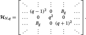 (18)
(18) Let us consider q =1/2 (we could alternatively take q =− 1/2) which makes the leading diagonal symmetric. We can then express this matrix Hamiltonian \(\widetilde {\mathcal {\boldsymbol {H}}}_{N} \equiv \boldsymbol {\mathcal {H}}_{N,q=1/2} \) in block form as
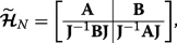 (19)
(19) Onde
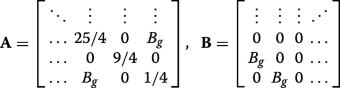 (20)
(20) are both of dimension N /2-by- N /2, and J is the exchange matrix. We may construct a matrix via permuting \(\boldsymbol {\mathcal {H}}_{N}\) with the N -by-N permutation matrix \(\boldsymbol {\mathcal {P}}_{N}\),
$$ \boldsymbol{\mathcal{P}}_{N} =\left[ \begin{array}{cccccc} 1 &0 &\hdots &\hdots &\hdots &0 \\ 0 &\hdots &\hdots &\hdots &\hdots &1 \\ 0 &1 &\hdots &\hdots &\hdots &0 \\ 0 &\hdots &\hdots &\hdots &1 &0 \\ \vdots &&&&&\vdots \\ 0 &\hdots &\hdots &1 &\hdots &0 \\ \end{array} \right], $$ (21)
such that the permutation-similar matrix is
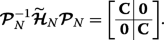 (22)
(22) Hence, the eigenvalues of \(\boldsymbol {\mathcal {P}}_{N}^{-1}\widetilde {\boldsymbol {\mathcal {H}}}_{N} \boldsymbol {\mathcal {P}}_{N}\), which are the same as the eigenvalues \(\widetilde {\boldsymbol {\mathcal {H}}}_{N}\), are double degenerate with the values given by the eigenvalue spectrum of the tridiagonal matrix C
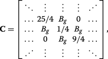 (23)
(23) which can also be expressed succinctly in terms of the previously defined matrices via \(\mathbf {C}=\boldsymbol {\mathcal {P}}_{N/2}^{-1}\mathbf {A}\boldsymbol {\mathcal {P}}_{N/2}+\boldsymbol {\mathcal {P}}_{N/2}^{-1}\mathbf {B}\mathbf {J}\boldsymbol {\mathcal {P}}_{N/2}^{4}\). We can see that applying C ⊥ ≠0 (inset of Fig. 3a) or both C ⊥ e A g ≠0 (inset of Fig. 3b) ruins the symmetry in the matrix Hamiltonian and prevents the existence of eigenvalues with multiplicity beyond unity, resulting in the appearance of band gaps.
Energy crossing at centre of Brillouin zone between third and forth subbands
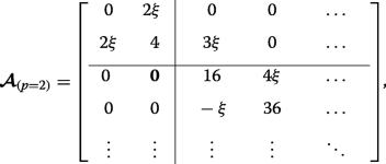
As an example, let us specifically consider the case where p =2, wherein the matrices (12) and (13) become:
 (24)
(24) e
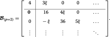 (25)
(25) This case corresponds to the crossings of the blue curves at the edge of the Brillouin zone in Fig. 3d (whereas p =0 results in crossings at q =0 in Fig. 3b). The lower eigenvalues are found exactly by diagonalizing each of the two finite matrices and they interlace, yielding \(\eta _{0,1,2} =2-\sqrt {4+4\xi ^{2}}, 4, 2+\sqrt {4+4\xi ^{2}}\). The infinite lower-right-hand block tridiagonal matrices coincide, thus the remaining double degenerate eigenvalues are found by approximately or numerically solving Det[D - η I ]=0.
Disponibilidade de dados e materiais
The data for the figures all stem from numerically diagonalizing the matrix described by Eq. 5 and can readily be achieved in any numerical software package. With this in mind, the datasets used and/or analyzed during the current study are available from the corresponding author on reasonable request.
Predição e análise eficientes de trapping óptico em nanoescala via elemento finito rasgando e método de interconexão
Nanopartículas híbridas magnéticas com nanopartículas de ouro funcionalizadas Her2:um agente teranóstico para imagem dual-modal e terapia fototérmica de câncer de mama
Nanomateriais