Um novo design de um sistema inteligente de administração de drogas baseado em partículas de nanoantena

Resumo

O sistema de distribuição de fármacos compostos por nanopartículas desempenha um papel importante na interação com os nódulos linfáticos. Existem três tipos principais de linfócitos:células B, células T e células assassinas naturais. Quando as células do sistema imunológico se tornam cancerígenas, elas atacam as células do corpo. O fluido linfático desempenha um papel importante no ataque às células saudáveis do corpo; portanto, este trabalho teve como objetivo projetar um sistema de entrega de drogas, que pode direcionar nanopartículas de forma eficiente para atingir as células infectadas, ajudando na eliminação em alta velocidade de tais células. O design proposto depende da interação entre essas moléculas, e o nano-controlador inteligente tem a capacidade de guiar as nanopartículas por contato anaeróbio. O projeto proposto provou que quanto menor o tamanho e a densidade das nanopartículas, menos dinâmica a viscosidade do líquido seria, o que refletiria sua resistência ao fluxo. Além disso, concluiu-se que as moléculas de hidrogênio desempenham um papel significativo na redução da resistência do fluido linfático devido à sua baixa densidade.

Introdução

As opções atuais de tratamento do câncer incluem cirurgia, radiação e quimioterapia. Essas estratégias de tratamento também prejudicam os tecidos comuns e resultam na aniquilação parcial do crescimento maligno. Portanto, a nanotecnologia pode superar essas deficiências, visando especificamente células prejudiciais e neoplasias, ressecando tumores diretamente e aumentando a eficácia da radiação e outras modalidades de tratamento. Isso pode diminuir significativamente os efeitos adversos do tratamento e aumentar a taxa de sobrevivência. A nanotecnologia é uma ferramenta promissora para o tratamento de crescimento maligno, pois oferece modalidades de tratamento mais novas e melhores com o uso de nanomateriais. As nanopartículas podem ter como alvo específico muitas moléculas expressas diferencialmente nas células cancerosas. A região geralmente vasta do aerofólio de nanopartículas pode ser funcionalizada com ligantes, tais como pequenas partículas e corrosivos desoxirribonucléicos ou anticorpos de peptídeos de cadeia corrosiva ribonucléica. Os ligantes são usados como fármaco e em aplicações teranósticas. As propriedades físicas das nanopartículas, como distração da vitalidade e re-irradiação, também podem ser usadas para afetar o tecido doente, como na remoção do laser e aplicações de hipertermia [1].

O programa de software inovador de nanopartículas e o elemento farmacêutico ativo também permitirão a exploração de um repertório mais amplo de ingredientes ativos. Portanto, a carga imunogênica e o revestimento de superfície estão sendo investigados como adjuvantes para quimioterapia mediada por nanopartículas e tradicional. Essa estratégia inovadora inclui o projeto de nanopartículas como antígenos artificiais que se apresentam nas células e depósitos in vivo de fatores estimuladores que exercem efeitos antitumorais. A nanotecnologia representa uma área ativa de pesquisa com muitas aplicações. As nanopartículas têm ganhado interesse na tecnologia médica devido às suas características físico-químicas ajustáveis, como ponto índice de descongelamento, hidrofilicidade, condução elétrica e térmica, atividade catalítica, absorção de luz e espalhamento [2]. Em princípio, os nanomateriais são descritos como materiais com partículas na faixa de 1 a 100 nm. Existem várias legislações na União Europeia e nos EUA com referência específica à investigação médica com nanomateriais. No entanto, não existe uma definição internacionalmente aceita de nanomateriais. Diferentes organizações consideram diferentes conceitos de nanomateriais [3]. Um dos objetivos do sistema de liberação de nanopartículas é tratar o fluido linfático com células cancerosas. Um sistema de distribuição de fármaco em nanopartículas de composto em interação com os nódulos linfáticos é mostrado na Fig. 1.

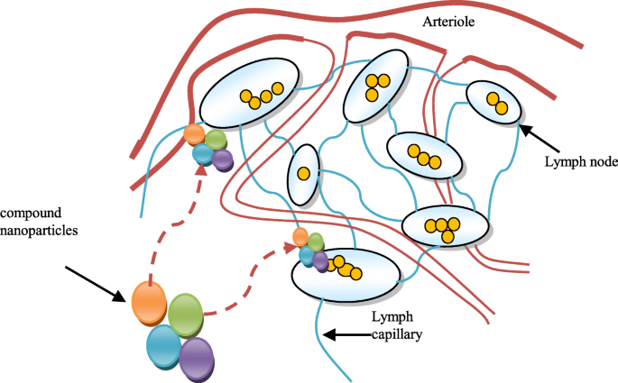
Sistema de distribuição de fármacos compostos de nanopartículas e sua interação com os nódulos linfáticos

A US Food and Drug Administration alude a nanomateriais como materiais com partículas na faixa de 1 a 100 com propriedades diferentes do material a granel [4, 5]. Nanofibras, nanoplacas, nanofios, pontos quânticos e outros materiais relacionados foram caracterizados [6]. Nanopartículas lipídicas sólidas (SLNs) são um tipo de nanopartículas lipídicas (LN), que podem ser construídas utilizando lipídeos sólidos [7]. Versões subsequentes de SLNs foram desenvolvidas, como portadores de lipídios nanoestruturados (NLCs), que representam a segunda era de LN [8]. Ambos SLN e NLC são construídos a partir de lipídios sólidos. A estrutura interna do SLN contém lipídios sólidos, enquanto o NLC é desenvolvido utilizando uma mistura de lipídios sólidos e líquidos, que produzem seções transversais de pedras preciosas [9, 10]. Essas falhas também foram relatadas para SLNs à luz do fato de que SLNs que contêm muitos segmentos de lipídios sólidos podem ser usados em aplicações médicas [11, 12]. Nanopartículas poliméricas (PN) podem ser construídas a partir de polímeros naturais ou materiais inorgânicos, por exemplo, sílica [13]. Os polímeros ou lipídios moldam o núcleo das NPs, que melhoram a estabilidade e a liberação da droga e oferecem forma e tamanho uniformes [14]. PN pode ser descrita como nanocápsulas ou nanoesferas. As nanocápsulas contêm óleo em uma estrutura vesicular junto com uma droga [15, 16], enquanto as nanoesferas contêm cadeias poliméricas sem óleo [17, 18]. Um medicamento é embalado em PNs por meio da mistura com o polímero. A incorporação do fármaco é garantida nas nanopartículas no momento da polimerização. Os PNs são carregados com uma droga dissolvendo, espalhando ou adsorvendo artificialmente nos constituintes da rede polimérica [19, 20]. Existem três tipos de linfócitos:células B, células T e células assassinas naturais. As células B produzem anticorpos que atacam os microorganismos invasores, enquanto também atacam o sistema imunológico quando se tornam cancerígenas. Portanto, considerando o importante papel do fluido linfático na autoimunidade, o objetivo deste trabalho foi projetar um sistema inteligente de liberação de fármacos baseado em partículas de nanoantena. Assim, o sistema contém muitas nanopartículas em diferentes quantidades. A próxima seção apresenta o projeto de um sistema inteligente de administração de medicamentos.

Projeto de um sistema nano-inteligente de administração de medicamentos

O sistema de entrega de drogas nano-inteligente proposto contém um nano-controlador operado por uma fonte elétrica de nanopartículas feitas de um material nano-piezoelétrico. O complexo repositório de nanopartículas possui vários micro-repositórios. Cada pequeno repositório contém um tipo de nanopartículas. Uma molécula de nanopartícula contém uma nanoantena projetada para se comunicar com o nano-controlador. O proposto sistema de entrega de drogas nanointeligente também contém nanotubos de carbono para a entrega rápida de drogas às células cancerosas. Ele pode ser associado às células infectadas, conforme mostrado na Fig. 2. O sistema começa enviando nanopartículas para as células cancerosas chamadas de "nanopartículas exploratórias". Essas moléculas, por meio da comunicação anaeróbia, enviam ao nanocontrolador o quadro completo de sua posição no interior das células. Com base na situação encontrada pelas nanopartículas exploratórias, o nano-controlador envia nanopartículas de número, tipo e densidade diferentes para as células cancerosas, com base nas informações coletadas das nanopartículas exploratórias. Essas nanopartículas são chamadas de "nanopartículas de combate".

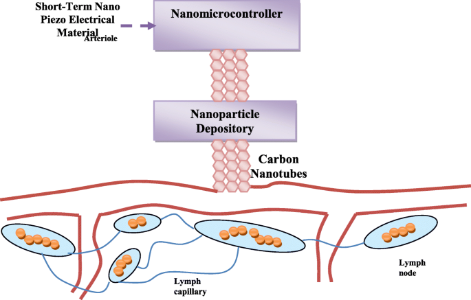
Estrutura geral mostrando a associação do sistema de drogas proposto com as células infectadas

Este não é um processo aleatório, mas controlado pelo nano-controlador considerando diversos aspectos e logaritmos, o que garantirá a entrega eficiente e rápida das nanopartículas. A fim de entregar com precisão e rapidez as nanopartículas às células cancerosas, o algoritmo de busca binária compressiva será empregado [21]. Além disso, as nanopartículas serão distribuídas em diferentes densidades para que a droga se torne mais eficaz. Essas metodologias e seu modus operandi empregando o nano-controlador são ilustrados na Fig. 3. A estrutura física do nano-controlador é semelhante à das nanopartículas, mas é na forma de metal para que possa ganhar energia elétrica por um curto período durante o trabalho. Este metal contém uma antena sem fio junto com uma pequena memória que contém os códigos operacionais com um link de nanopartículas entre o nano-controlador e o armazenamento de nanopartículas. O repositório de nanopartículas contém vários tipos diferentes de nanopartículas. A abertura e o fechamento, bem como a duração da abertura do nano-gate, serão controlados para ajustar o número de partículas a serem entregues.

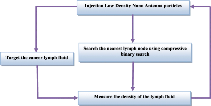
Processo de envio das nanopartículas de combate às células cancerosas

Uma descrição da natureza das nanopartículas usadas no sistema de medicamentos proposto

Na próxima seção, a natureza das nanopartículas utilizadas no sistema de entrega de drogas proposto é discutida. Neste trabalho, nanopartículas anaeróbicas de baixa densidade foram usadas conforme descrito em um relatório anterior [22].

Nanopartículas de baixa densidade

Considere o processo de entrega de drogas de nanopartículas compostas para o câncer como um processo de penetração no fluido linfático, onde um tumor é circundado pelo fluido linfático. A composição do melanoma se assemelha ao fluido linfático. O modelo analítico proposto é baseado em um sistema de nanotubos constituído por três tipos diferentes de nanopartículas. As nanopartículas são colocadas em um fluido linfático de alta densidade. Podemos definir nanopartículas específicas do sólido A nas coordenadas polares esféricas como A =(Ra, ϑ a , φa), onde ra é a coordenada radial para a nanopartícula do sólido A, ϑ a é a coordenada zenital para a nanopartícula do sólido A, e φa é a coordenada azimutal para a nanopartícula do sólido A. As coordenadas correspondentes do sólido B são B =(Rb, ϑb, φb), respectivamente, e as coordenadas correspondentes de N sólido são N =(Rn, ϑn, φn), respectivamente. Considere que existem duas propriedades do linfonodo, viz., Sensível e inchado, que são afetadas pelas células cancerosas do linfoma de Hodgkin. O linfonodo com propriedade sensível Tp pode ser descrito como Tp ( N , t ); isso significa que o valor de Tp em associação com o fluido de nanopartículas de N sólido varia com o tempo. Agora, vamos considerar que o efeito total das nanopartículas compostas na propriedade de concurso é definido como:
$$ \ mathrm {Tpt} =\ mathrm {Tp} \ \ left (A, t \ right) + \ mathrm {Tp} \ \ left (B, t \ right) +. \ dots \ dots \ dots \ dots + \ mathrm {Tp} \ \ left (N, t \ right) $$ (1)
Considere o mesmo caso para a propriedade inchada, que pode ser definida como:
$$ \ mathrm {Tst} =\ mathrm {Ts} \ \ left (A, t \ right) + \ mathrm {Ts} \ \ left (B, t \ right) +. \ dots \ dots \ dots \ dots + \ mathrm {Ts} \ \ left (N, t \ right) $$ (2)
Das Eqs. 1 e 2, a taxa de mudança de ambas as propriedades com o tempo pode ser determinada como:
$$ \ frac {\ partial \ left (\ mathrm {Tp} \ left (A, t \ right) \ right)} {\ partial t} + \ frac {\ partial \ left (\ mathrm {Tp} \ left ( B, t \ right) \ right)} {\ partial t} + \ dots \ frac {\ partial \ left (\ mathrm {Tp} \ left (N, t \ right) \ right)} {\ partial t} =\ frac {\ mathrm {\ partial Tp} (t)} {\ mathrm {\ partial t}} $$ (3) $$ \ frac {\ partial \ left (\ mathrm {Ts} \ left (A, t \ direita) \ direita)} {\ parcial t} + \ frac {\ parcial \ esquerda (\ mathrm {Ts} \ esquerda (B, t \ direita) \ direita)} {\ parcial t} + \ pontos \ frac {\ parcial \ esquerda (\ mathrm {Ts} \ esquerda (N, t \ direita) \ direita)} {\ parcial t} =\ frac {\ mathrm {\ parcial Ts} (t)} {\ parcial t} $$ ( 4)
O ponto no fluido linfático que pode ser ocupado por uma nanopartícula de N sólido é definido como:
$$ {\ mathrm {Po}} _ n =\ mathrm {Po} {\ left (\ mathrm {po}, t \ right)} _ n $$ (5)
Vamos considerar que uma nanopartícula do derivado N sólido do fluido linfático macio é definida como \ (\ frac {\ partial {\ left (\ mathrm {Tp} \ left (N, t \ right) \ right)} _ {\ mathrm {po}}} {\ partial t} \), então o material composto derivado do fluido linfático sensível seria igual a:
$$ \ frac {\ partial {\ left (\ mathrm {Tp} \ left (A, t \ right) \ right)} _ {\ mathrm {po}}} {\ partial t} + \ frac {\ partial { \ left (\ mathrm {Tp} \ left (B, t \ right) \ right)} _ {\ mathrm {po}}} {\ partial t} + \ dots \ frac {\ partial {\ left (\ mathrm { Tp} \ left (N, t \ right) \ right)} _ {\ mathrm {po}}} {\ partial t} =\ frac {\ mathrm {\ partial Tp} {(t)} _ {\ mathrm { po}}} {\ partial t} $$ (6) $$ \ frac {\ partial {\ left (\ mathrm {Ts} \ left (A, t \ right) \ right)} _ {\ mathrm {po} }} {\ partial t} + \ frac {\ partial {\ left (\ mathrm {Ts} \ left (B, t \ right) \ right)} _ {\ mathrm {po}}} {\ partial t} + \ dots \ frac {\ partial {\ left (\ mathrm {Ts} \ left (N, t \ right) \ right)} _ {\ mathrm {po}}} {\ partial t} =\ frac {\ mathrm { \ parcial Ts} {(t)} _ {\ mathrm {po}}} {\ parcial t} $$ (7)
Os componentes de velocidade correspondentes do sólido N são considerados como ( v _rn , v _ϑn , v _φn ) Então, a velocidade do fluxo das partículas de N sólido é representada usando as equações de Navier-Stokes na viscosidade dinâmica dν do fluido linfático, e p é a pressão e ρ é a densidade do fluido linfático da seguinte forma:
$$ \ frac {\ parcial {v} _ {\ mathrm {rn}}} {\ parcial t} + {v} _ {\ mathrm {rn}} \ frac {\ parcial {v} _ {\ mathrm {rn }}} {\ mathrm {\ partial rn}} + \ frac {v _ {\ upvartheta \ mathrm {n}}} {\ mathrm {rn}} \ frac {\ partial {v} _ {\ mathrm {rn}} } {\ mathrm {\ partial \ upvartheta n}} + \ frac {v _ {\ upvarphi \ mathrm {n}}} {\ mathrm {rn} \ \ mathrm {sin} \ upvartheta \ mathrm {n}} \ frac { \ parcial {v} _ {\ mathrm {rn}}} {\ mathrm {\ partial \ upvarphi n}} - \ frac {v _ {\ upvartheta \ mathrm {n}} ^ 2} {\ mathrm {rn}} - \ frac {v _ {\ upvarphi \ mathrm {n}} ^ 2} {\ mathrm {rn}} + \ frac {1} {\ rho} \ frac {\ partial p} {\ mathrm {\ partial rn}} - \ mathrm {d} \ upnu \ left [\ frac {1} {{\ mathrm {rn}} ^ 2} \ frac {\ partial} {\ mathrm {\ partial rn}} \ left ({\ mathrm {rn} } ^ 2 \ frac {\ partial {v} _ {\ mathrm {rn}}} {\ mathrm {\ partial rn}} \ right) + \ frac {1} {{\ mathrm {rn}} ^ 2 \ mathrm {sin} \ upvartheta \ mathrm {n}} \ frac {\ partial} {\ mathrm {\ partial \ upvartheta n}} \ left (\ mathrm {sin} \ upvartheta \ mathrm {n} \ frac {\ partial {v } _ {\ mathrm {rn}}} {\ mathrm {\ partial \ upvartheta n}} \ right) + \ frac {1} {{\ mathrm {rn}} ^ 2 {\ sin} ^ 2 \ upvartheta \ mathrm {n}} \ frac {\ partial ^ 2 {v} _ {\ ma thrm {rn}}} {\ partial {\ upvarphi \ mathrm {n}} ^ 2} + - \ frac {2 {v} _ {\ mathrm {rn}}} {{\ mathrm {rn}} ^ 2} - \ frac {2} {{\ mathrm {rn}} ^ 2 \ sin \ upvartheta \ mathrm {n}} \ frac {\ partial \ left ({v} _ {\ upvartheta \ mathrm {n}} \ mathrm { sin} \ upvartheta \ mathrm {n} \ right)} {\ mathrm {\ partial \ upvartheta n}} - \ frac {2} {{\ mathrm {rn}} ^ 2 \ mathrm {sin} \ upvartheta \ mathrm { n}} \ frac {\ partial {v} _ {\ upvarphi \ mathrm {n}}} {\ partial _ {\ upvarphi \ mathrm {n}}} \ right] =0 $$ (8)
A viscosidade dinâmica dν do fluido linfático é calculada da seguinte forma:
$$ \ mathrm {d} \ upnu =\ frac {\ left [\ frac {\ parcial {v} _ {\ mathrm {rn}}} {\ parcial t} + {v} _ {\ mathrm {rn}} \ frac {\ parcial {v} _ {\ mathrm {rn}}} {\ mathrm {\ parcial rn}} + \ frac {v _ {\ upvartheta \ mathrm {n}} \ parcial {v} _ {\ mathrm { rn}}} {\ mathrm {rn} \ \ mathrm {\ partial \ upvartheta n}} + \ frac {v _ {\ upvarphi \ mathrm {n}}} {\ mathrm {rn} \ \ mathrm {sin} \ upvartheta \ mathrm {n}} \ frac {\ partial {v} _ {\ mathrm {rn}}} {\ mathrm {\ partial \ upvarphi n}} - \ frac {v _ {\ upvartheta \ mathrm {n}} ^ 2 } {\ mathrm {rn}} - \ frac {v _ {\ upvarphi \ mathrm {n}} ^ 2} {\ mathrm {rn}} + \ frac {1 \ \ partial p} {\ uprho \ partial \ mathrm { rn}} \ right]} {\ left [\ frac {1} {{\ mathrm {rn}} ^ 2} \ frac {\ partial} {\ mathrm {\ partial rn}} \ left ({\ mathrm {rn }} ^ 2 \ frac {\ partial {v} _ {\ mathrm {rn}}} {\ mathrm {\ partial rn}} \ right) + \ frac {1} {{\ mathrm {rn}} ^ 2 \ mathrm {sin} \ upvartheta \ mathrm {n}} \ frac {\ partial} {\ mathrm {\ partial \ upvartheta n}} \ left (\ mathrm {sin} \ upvartheta \ mathrm {n} \ frac {\ partial { v} _ {\ mathrm {rn}}} {\ mathrm {\ partial \ upvartheta n}} \ right) + \ frac {1} {{\ mathrm {rn}} ^ 2 {\ sin} ^ 2 \ upvartheta \ mathrm {n}} \ frac {\ parcial ^ 2 {v} _ {\ mathrm {rn}}} {\ parcial {\ upvarphi \ mathrm {n}} ^ 2} + - \ frac {2 {v} _ {\ mathrm {rn}}} {{\ mathrm {rn}} ^ 2} - \ frac {2} {{\ mathrm {rn}} ^ 2 \ sin \ upvartheta \ mathrm {n}} \ frac {\ partial \ left ({v} _ {\ upvartheta \ mathrm {n}} \ mathrm {sin} \ upvartheta \ mathrm {n} \ right)} {\ mathrm {\ partial \ upvartheta n}} - \ frac {2} {{\ mathrm {rn}} ^ 2 \ mathrm {sin} \ upvartheta \ mathrm {n}} \ frac {\ partial {v} _ {\ upvarphi \ mathrm {n}}} {\ partial _ {\ upvarphi \ mathrm {n}}} \ right]} $$ ( 9)
As equações de Navier-Stokes dos sólidos A e B podem ser representadas como Eqs. 8 e 9. Assim, a Eq. 9 pode ser representado da seguinte forma:
$$ \ mathrm {d} \ upnu =\ frac {\ left [\ frac {\ parcial {v} _ {\ mathrm {rn}}} {\ parcial t} + {v} _ {\ mathrm {rn}} \ frac {\ parcial {v} _ {\ mathrm {rn}}} {\ mathrm {\ parcial rn}} + \ frac {v _ {\ upvartheta \ mathrm {n}}} {\ mathrm {rn}} \ frac {\ partial {v} _ {\ mathrm {rn}}} {\ mathrm {\ partial \ upvartheta n}} + \ frac {v _ {\ upvarphi \ mathrm {n}}} {\ mathrm {rn} \ \ mathrm {sin} \ upvartheta \ mathrm {n}} \ frac {\ partial {v} _ {\ mathrm {rn}}} {\ mathrm {\ partial \ upvarphi n}} - \ frac {v _ {\ upvartheta \ mathrm { n}} ^ 2} {\ mathrm {rn}} - \ frac {v _ {\ upvarphi \ mathrm {n}} ^ 2} {\ mathrm {rn}} + \ frac {1} {\ rho} \ frac { \ parcial p} {\ mathrm {\ partial rn}} \ right]} {\ left [\ frac {1} {{\ mathrm {rn}} ^ 2} \ frac {\ partial} {\ mathrm {\ partial rn }} \ left ({\ mathrm {rn}} ^ 2 \ frac {\ partial {v} _ {\ mathrm {rn}}} {\ mathrm {\ partial rn}} \ right) + \ frac {1} { {\ mathrm {rn}} ^ 2 \ mathrm {sin} \ upvartheta \ mathrm {n}} \ frac {\ partial} {\ mathrm {\ partial \ upvartheta n}} \ left (\ mathrm {sin} \ upvartheta \ mathrm {n} \ frac {\ partial {\ mathrm {v}} _ {\ mathrm {rn}}} {\ mathrm {\ partial \ upvartheta n}} \ right) + \ frac {1} {{\ mathrm { rn}} ^ 2 {\ sin} ^ 2 \ upvartheta \ math rm {n}} \ frac {\ partial ^ 2 {\ mathrm {v}} _ {\ mathrm {rn}}} {\ partial {\ upvarphi \ mathrm {n}} ^ 2} - \ frac {2 {\ mathrm {v}} _ {\ mathrm {rn}}} {{\ mathrm {rn}} ^ 2} - \ frac {2} {{\ mathrm {rn}} ^ 2 \ sin \ upvartheta \ mathrm {n} } \ frac {\ partial \ left ({\ mathrm {v}} _ {\ upvartheta \ mathrm {n}} \ mathrm {sin} \ upvartheta \ mathrm {n} \ right)} {\ mathrm {\ partial \ upvartheta n}} - \ frac {2} {{\ mathrm {rn}} ^ 2 \ mathrm {sin} \ upvartheta \ mathrm {n}} \ frac {\ partial {\ mathrm {v}} _ {\ upvarphi \ mathrm {n}}} {\ partial _ {\ upvarphi \ mathrm {n}}} \ right]} =\ frac {\ left [\ frac {\ partial {\ mathrm {v}} _ {\ mathrm {ra}}} {\ mathrm {\ partial t}} + {\ mathrm {v}} _ {\ mathrm {ra}} \ frac {\ partial {\ mathrm {v}} _ {\ mathrm {ra}}} {\ mathrm { \ parcial ra}} + \ frac {{\ mathrm {v}} _ {\ upvartheta \ mathrm {a}}} {\ mathrm {ra}} \ frac {\ parcial {\ mathrm {v}} _ {\ mathrm {ra}}} {\ mathrm {\ partial \ upvartheta a}} + \ frac {{\ mathrm {v}} _ {\ upvarphi \ mathrm {a}}} {\ mathrm {ra} \ \ mathrm {sin} \ upvartheta \ mathrm {a}} \ frac {\ partial {\ mathrm {v}} _ {\ mathrm {ra}}} {\ mathrm {\ partial \ upvarphi a}} - \ frac {{\ mathrm {v} } _ {\ upvartheta \ mathrm {a}} ^ 2} {\ mathrm {ra}} - \ frac {{\ mathrm {v}} _ {\ upvarphi \ mathrm {a}} ^ 2} {\ mathrm {ra}} + \ frac {1} {\ uprho} \ frac {\ mathrm {\ partial p} } {\ mathrm {\ partial ra}} \ right]} {\ left [\ frac {1} {{\ mathrm {ra}} ^ 2} \ frac {\ partial} {\ mathrm {\ partial ra}} \ esquerda ({\ mathrm {ra}} ^ 2 \ frac {\ parcial {v} _ {\ mathrm {ra}}} {\ mathrm {\ parcial ra}} \ direita) + \ frac {1} {{\ mathrm {ra}} ^ 2 \ mathrm {sin} \ upvartheta \ mathrm {a}} \ frac {\ partial} {\ mathrm {\ partial \ upvartheta a}} \ left (\ mathrm {sin} \ upvartheta \ mathrm {a } \ frac {\ partial {v} _ {\ mathrm {ra}}} {\ mathrm {\ partial \ upvartheta a}} \ right) + \ frac {1} {{\ mathrm {ra}} ^ 2 {\ sin} ^ 2 \ upvartheta \ mathrm {a}} \ frac {\ partial ^ 2 {v} _ {\ mathrm {ra}}} {\ partial {\ upvarphi \ mathrm {a}} ^ 2} - \ frac { 2 {v} _ {\ mathrm {ra}}} {{\ mathrm {ra}} ^ 2} - \ frac {2} {{\ mathrm {ra}} ^ 2 \ sin \ upvartheta \ mathrm {a}} \ frac {\ partial \ left ({v} _ {\ upvartheta \ mathrm {a}} \ mathrm {sin} \ upvartheta \ mathrm {a} \ right)} {\ mathrm {\ partial \ upvartheta a}} - \ frac {2} {{\ mathrm {ra}} ^ 2 \ mathrm {sin} \ upvartheta \ mathrm {a}} \ frac {\ partial {v} _ {\ upvarphi \ mathrm {a}}} {\ partial_ { \ upvarphi \ mathrm {a}}} \ right]} =\ frac { \ left [\ frac {\ partial {v} _ {\ mathrm {rb}}} {\ partial t} + {v} _ {\ mathrm {rb}} \ frac {\ partial {v} _ {\ mathrm { rb}}} {\ mathrm {\ partial rb}} + \ frac {v _ {\ upvartheta \ mathrm {b}}} {\ mathrm {rb}} \ frac {\ partial {v} _ {\ mathrm {rb} }} {\ mathrm {\ partial \ upvartheta b}} + \ frac {v _ {\ upvarphi \ mathrm {b}}} {\ mathrm {rb} \ \ mathrm {sin} \ upvartheta \ mathrm {b}} \ frac {\ partial {v} _ {\ mathrm {rb}}} {\ mathrm {\ partial \ upvarphi b}} - \ frac {v _ {\ upvartheta \ mathrm {b}} ^ 2} {\ mathrm {rb}} - \ frac {v _ {\ upvarphi \ mathrm {b}} ^ 2} {\ mathrm {rb}} + \ frac {1} {\ rho} \ frac {\ partial p} {\ mathrm {\ partial rb}} \ right]} {\ left [\ frac {1} {{\ mathrm {rb}} ^ 2} \ frac {\ partial} {\ mathrm {\ partial rb}} \ left ({\ mathrm {rb}} ^ 2 \ frac {\ partial {v} _ {\ mathrm {rb}}} {\ mathrm {\ partial rb}} \ right) + \ frac {1} {{\ mathrm {rb}} ^ 2 \ mathrm {sin } \ upvartheta \ mathrm {b}} \ frac {\ parcial} {\ mathrm {\ parcial \ upvartheta b}} \ left (\ mathrm {sin} \ upvartheta \ mathrm {b} \ frac {\ parcial {v} _ {\ mathrm {rb}}} {\ mathrm {\ partial \ upvartheta b}} \ right) + \ frac {1} {{\ mathrm {rb}} ^ 2 {\ sin} ^ 2 \ upvartheta \ mathrm {b }} \ frac {\ partial ^ 2 {v} _ {\ mathrm { rb}}} {\ partial {\ upvarphi \ mathrm {b}} ^ 2} - \ frac {2 {v} _ {\ mathrm {rb}}} {{\ mathrm {rb}} ^ 2} - \ frac {2} {{\ mathrm {rb}} ^ 2 \ sin \ upvartheta \ mathrm {b}} \ frac {\ partial \ left ({v} _ {\ upvartheta \ mathrm {b}} \ mathrm {sin} \ upvartheta \ mathrm {b} \ right)} {\ mathrm {\ partial \ upvartheta b}} - \ frac {2} {{\ mathrm {rb}} ^ 2 \ mathrm {sin} \ upvartheta \ mathrm {b}} \ frac {\ partial {v} _ {\ upvarphi \ mathrm {b}}} {\ partial _ {\ upvarphi \ mathrm {b}}} \ right]} $$ (10)
As partículas estão em nanodimensões; assim, seus raios seriam muito pequenos e, para simplificar, a Eq. 10 é representado da seguinte forma:
$$ \ mathrm {d} \ upnu =\ left [\ frac {v _ {\ upvartheta \ mathrm {n}}} {\ mathrm {rn}} \ frac {\ partial {v} _ {\ mathrm {rn}} } {\ mathrm {\ partial \ upvartheta n}} + \ frac {v _ {\ upvarphi \ mathrm {n}}} {\ mathrm {rn} \ \ mathrm {sin} \ upvartheta \ mathrm {n}} \ frac { \ parcial {v} _ {\ mathrm {rn}}} {\ mathrm {\ partial \ upvarphi n}} - \ frac {v _ {\ upvartheta \ mathrm {n}} ^ 2} {\ mathrm {rn}} - \ frac {v _ {\ upvarphi \ mathrm {n}} ^ 2} {\ mathrm {rn}} + \ frac {1} {\ rho} \ frac {\ partial p} {\ mathrm {\ partial rn}} \ direita] / \ esquerda [\ frac {1} {{\ mathrm {rn}} ^ 2} \ frac {\ partial} {\ mathrm {\ partial rn}} \ left ({\ mathrm {rn}} ^ 2 \ frac {\ partial {v} _ {\ mathrm {rn}}} {\ mathrm {\ partial rn}} \ right) + \ frac {1} {{\ mathrm {rn}} ^ 2 \ mathrm {sin} \ upvartheta \ mathrm {n}} \ frac {\ partial} {\ mathrm {\ partial \ upvartheta n}} \ left (\ mathrm {sin} \ upvartheta \ mathrm {n} \ frac {\ partial {\ mathrm {v} } _ {\ mathrm {rn}}} {\ mathrm {\ partial \ upvartheta n}} \ right) + \ frac {1} {{\ mathrm {rn}} ^ 2 {\ sin} ^ 2 \ upvartheta \ mathrm {n}} \ frac {\ partial ^ 2 {\ mathrm {v}} _ {\ mathrm {rn}}} {\ partial {\ upvarphi \ mathrm {n}} ^ 2} - \ frac {2 {\ mathrm {v}} _ {\ mathrm {rn}}} {{\ math rm {rn}} ^ 2} - \ frac {2} {{\ mathrm {rn}} ^ 2 \ sin \ upvartheta \ mathrm {n}} \ frac {\ partial \ left ({\ mathrm {v}} _ {\ upvartheta \ mathrm {n}} \ mathrm {sin} \ upvartheta \ mathrm {n} \ right)} {\ mathrm {\ partial \ upvartheta n}} - \ frac {2} {{\ mathrm {rn}} ^ 2 \ mathrm {sin} \ upvartheta \ mathrm {n}} \ frac {\ partial {\ mathrm {v}} _ {\ upvarphi \ mathrm {n}}} {\ partial _ {\ upvarphi \ mathrm {n}} } \ right] =\ left [\ frac {{\ mathrm {v}} _ {\ upvartheta \ mathrm {a}}} {\ mathrm {ra}} \ frac {\ partial {\ mathrm {v}} _ { \ mathrm {ra}}} {\ mathrm {\ partial \ upvartheta a}} + \ frac {{\ mathrm {v}} _ {\ upvarphi \ mathrm {a}}} {\ mathrm {ra} \ \ mathrm { sin} \ upvartheta \ mathrm {a}} \ frac {\ partial {\ mathrm {v}} _ {\ mathrm {ra}}} {\ mathrm {\ partial \ upvarphi a}} - \ frac {{\ mathrm { v}} _ {\ upvartheta \ mathrm {a}} ^ 2} {\ mathrm {ra}} - \ frac {{\ mathrm {v}} _ {\ upvarphi \ mathrm {a}} ^ 2} {\ mathrm {ra}} + \ frac {1} {\ uprho} \ frac {\ mathrm {\ partial p}} {\ mathrm {\ partial ra}} \ right] / \ left [\ frac {1} {{\ mathrm {ra}} ^ 2} \ frac {\ partial} {\ mathrm {\ partial ra}} \ left ({\ mathrm {ra}} ^ 2 \ frac {\ partial {\ mathrm {v}} _ {\ mathrm {ra}}} {\ mathrm {\ partial ra}} \ rig ht) + \ frac {1} {{\ mathrm {ra}} ^ 2 \ mathrm {sin} \ upvartheta \ mathrm {a}} \ frac {\ partial} {\ mathrm {\ partial \ upvartheta a}} \ left (\ mathrm {sin} \ upvartheta \ mathrm {a} \ frac {\ partial {\ mathrm {v}} _ {\ mathrm {ra}}} {\ mathrm {\ partial \ upvartheta a}} \ right) + \ frac {1} {{\ mathrm {ra}} ^ 2 {\ sin} ^ 2 \ upvartheta \ mathrm {a}} \ frac {\ partial ^ 2 {\ mathrm {v}} _ {\ mathrm {ra}} } {\ partial {\ upvarphi \ mathrm {a}} ^ 2} - \ frac {2 {\ mathrm {v}} _ {\ mathrm {ra}}} {{\ mathrm {ra}} ^ 2} - \ frac {2} {{\ mathrm {ra}} ^ 2 \ sin \ upvartheta \ mathrm {a}} \ frac {\ partial \ left ({\ mathrm {v}} _ {\ upvartheta \ mathrm {a}} \ mathrm {sin} \ upvartheta \ mathrm {a} \ right)} {\ mathrm {\ partial \ upvartheta a}} - \ frac {2} {{\ mathrm {ra}} ^ 2 \ mathrm {sin} \ upvartheta \ mathrm {a}} \ frac {\ partial {v} _ {\ upvarphi \ mathrm {a}}} {\ partial _ {\ upvarphi \ mathrm {a}}} \ right] =\ left [\ frac {v _ {\ upvartheta \ mathrm {b}}} {\ mathrm {rb}} \ frac {\ partial {v} _ {\ mathrm {rb}}} {\ mathrm {\ partial \ upvartheta b}} + \ frac {v _ {\ upvarphi \ mathrm {b}}} {\ mathrm {rb} \ \ mathrm {sin} \ upvartheta \ mathrm {b}} \ frac {\ partial {v} _ {\ mathrm {rb}}} {\ mathrm {\ parcial \ upvarphi b}} - \ frac {v _ {\ upvartheta \ mathrm {b}} ^ 2} {\ mathrm {rb}} - \ frac {v _ {\ upvarphi \ mathrm {b}} ^ 2} {\ mathrm {rb }} + \ frac {1} {\ rho} \ frac {\ partial p} {\ mathrm {\ partial rb}} \ right] / \ left [\ frac {1} {{\ mathrm {rb}} ^ 2 } \ frac {\ partial} {\ mathrm {\ partial rb}} \ left ({\ mathrm {rb}} ^ 2 \ frac {\ partial {v} _ {\ mathrm {rb}}} {\ mathrm {\ parcial rb}} \ right) + \ frac {1} {{\ mathrm {rb}} ^ 2 \ mathrm {sin} \ upvartheta \ mathrm {b}} \ frac {\ partial} {\ mathrm {\ partial \ upvartheta b}} \ left (\ mathrm {sin} \ upvartheta \ mathrm {b} \ frac {\ partial {v} _ {\ mathrm {rb}}} {\ mathrm {\ partial \ upvartheta b}} \ right) + \ frac {1} {{\ mathrm {rb}} ^ 2 {\ sin} ^ 2 \ upvartheta \ mathrm {b}} \ frac {\ partial ^ 2 {v} _ {\ mathrm {rb}}} {\ parcial {\ upvarphi \ mathrm {b}} ^ 2} - \ frac {2 {v} _ {\ mathrm {rb}}} {{\ mathrm {rb}} ^ 2} - \ frac {2} {{\ mathrm {rb}} ^ 2 \ sin \ upvartheta \ mathrm {b}} \ frac {\ partial \ left ({v} _ {\ upvartheta \ mathrm {b}} \ mathrm {sin} \ upvartheta \ mathrm {b} \ right)} {\ mathrm {\ partial \ upvartheta b}} - \ frac {2} {{\ mathrm {rb}} ^ 2 \ mathrm {sin} \ upvartheta \ mathrm {b}} \ frac {\ partial { v} _ {\ upvarphi \ mathrm {b}}} {\ parcial _ {\ upvarphi \ mathrm {b}}} \ right] $$ (11)
A Equação 11 pode ser representada da seguinte forma:
$$ \ mathrm {d} \ upnu =\ mathrm {rn} \ left [{v} _ {\ upvartheta \ mathrm {n}} \ frac {\ partial {v} _ {\ mathrm {rn}}} {\ mathrm {\ partial \ upvartheta n}} + \ frac {v _ {\ upvarphi \ mathrm {n}}} {\ \ mathrm {sin} \ upvartheta \ mathrm {n}} \ frac {\ partial {v} _ {\ mathrm {rn}}} {\ mathrm {\ partial \ upvarphi n}} - {v} _ {\ upvartheta \ mathrm {n}} ^ 2- {v} _ {\ upvarphi \ mathrm {n}} ^ 2+ \ frac {\ mathrm {rn}} {\ rho} \ frac {\ partial p} {\ mathrm {\ partial rn}} \ right] / \ left [\ frac {\ partial} {\ mathrm {\ partial rn} } \ left ({\ mathrm {rn}} ^ 2 \ frac {\ partial {v} _ {\ mathrm {rn}}} {\ mathrm {\ partial rn}} \ right) + \ frac {1} {\ mathrm {sin} \ upvartheta \ mathrm {n}} \ frac {\ partial} {\ mathrm {\ partial \ upvartheta n}} \ left (\ mathrm {sin} \ upvartheta \ mathrm {n} \ frac {\ partial { v} _ {\ mathrm {rn}}} {\ mathrm {\ parcial \ upvartheta n}} \ direita) + \ frac {1} {\ sin ^ 2 \ upvartheta \ mathrm {n}} \ frac {\ parcial ^ 2 {v} _ {\ mathrm {rn}}} {\ parcial {\ upvarphi \ mathrm {n}} ^ 2} -2 {v} _ {\ mathrm {rn}} - \ frac {2} {\ sin \ upvartheta \ mathrm {n}} \ frac {\ partial \ left ({v} _ {\ upvartheta \ mathrm {n}} \ mathrm {sin} \ upvartheta \ mathrm {n} \ right)} {\ mathrm {\ par tial \ upvartheta n}} - \ frac {2} {\ mathrm {sin} \ upvartheta \ mathrm {n}} \ frac {\ partial {v} _ {\ upvarphi \ mathrm {n}}} {\ partial _ {\ upvarphi \ mathrm {n}}} \ right] =\ mathrm {ra} \ left [{v} _ {\ upvartheta \ mathrm {a}} \ frac {\ partial {v} _ {\ mathrm {ra}}} {\ mathrm {\ partial \ upvartheta a}} + \ frac {v _ {\ upvarphi \ mathrm {a}}} {\ \ mathrm {sin} \ upvartheta \ mathrm {a}} \ frac {\ partial {v} _ {\ mathrm {ra}}} {\ mathrm {\ partial \ upvarphi a}} - {v} _ {\ upvartheta \ mathrm {a}} ^ 2- {v} _ {\ upvarphi \ mathrm {a}} ^ 2+ \ frac {\ mathrm {ra}} {\ rho} \ frac {\ partial p} {\ mathrm {\ partial ra}} \ right] / \ left [\ frac {\ partial} {\ mathrm {\ partial ra}} \ left ({\ mathrm {ra}} ^ 2 \ frac {\ partial {v} _ {\ mathrm {ra}}} {\ mathrm {\ partial ra}} \ right) + \ frac {1} {\ mathrm {sin} \ upvartheta \ mathrm {a}} \ frac {\ partial} {\ mathrm {\ partial \ upvartheta a}} \ left (\ mathrm {sin} \ upvartheta \ mathrm {a} \ frac {\ parcial {v} _ {\ mathrm {ra}}} {\ mathrm {\ parcial \ upvartheta a}} \ direita) + \ frac {1} {\ sin ^ 2 \ upvartheta \ mathrm {a}} \ frac {\ parcial ^ 2 {v} _ {\ mathrm {ra}}} {\ parcial {\ upvarphi \ mathrm {a}} ^ 2} -2 {v} _ {\ mathrm {ra}} - \ frac {2} { \pecado \ upvartheta \ mathrm {a}} \ frac {\ partial \ left ({v} _ {\ upvartheta \ mathrm {a}} \ mathrm {sin} \ upvartheta \ mathrm {a} \ right)} {\ mathrm {\ parcial \ upvartheta a}} - \ frac {2} {\ mathrm {sin} \ upvartheta \ mathrm {a}} \ frac {\ parcial {v} _ {\ upvarphi \ mathrm {a}}} {\ parcial _ {\ upvarphi \ mathrm {a}}} \ right] =\ mathrm {rb} \ left [{v} _ {\ upvartheta \ mathrm {b}} \ frac {\ partial {v} _ {\ mathrm {rb}}} {\ mathrm {\ partial \ upvartheta b}} + \ frac {v _ {\ upvarphi \ mathrm {b}}} {\ \ mathrm {sin} \ upvartheta \ mathrm {b}} \ frac {\ partial {v} _ {\ mathrm {rb}}} {\ mathrm {\ partial \ upvarphi b}} - {v} _ {\ upvartheta \ mathrm {b}} ^ 2- {v} _ {\ upvarphi \ mathrm {b}} ^ 2+ \ frac {\ mathrm {rb}} {\ rho} \ frac {\ partial p} {\ mathrm {\ partial rb}} \ right] / \ left [\ frac {\ partial} {\ mathrm {\ partial rb}} \ left ({\ mathrm {rb}} ^ 2 \ frac {\ partial {v} _ {\ mathrm {rb}}} {\ mathrm {\ partial rb}} \ right) + \ frac {1} {\ mathrm {sin} \ upvartheta \ mathrm {b}} \ frac {\ parcial} {\ mathrm {\ parcial \ upvartheta b}} \ left (\ mathrm {sin} \ upvartheta \ mathrm {b} \ frac {\ parcial {v} _ {\ mathrm {rb}}} {\ mathrm {\ partial \ upvartheta b}} \ right) + \ frac {1} {\ si n ^ 2 \ upvartheta \ mathrm {b}} \ frac {\ partial ^ 2 {v} _ {\ mathrm {rb}}} {\ partial {\ upvarphi \ mathrm {b}} ^ 2} -2 {v} _ {\ mathrm {rb}} - \ frac {2} {\ sin \ upvartheta \ mathrm {b}} \ frac {\ partial \ left ({v} _ {\ upvartheta \ mathrm {b}} \ mathrm {sin } \ upvartheta \ mathrm {b} \ right)} {\ mathrm {\ partial \ upvartheta b}} - \ frac {2} {\ mathrm {sin} \ upvartheta \ mathrm {b}} \ frac {\ partial {v } _ {\ upvarphi \ mathrm {b}}} {\ partial _ {\ upvarphi \ mathrm {b}}} \ right] $$ (12)
Existe uma relação direta entre os raios das nanopartículas e a viscosidade da linfa devido ao câncer. Se a linfa se torna muito estática e viscosa, ela é incapaz de realizar sua função adequadamente, que é a de circular e limpar toxinas e ajudar a combater o câncer. Se o tamanho das nanopartículas for menor, as células cancerosas linfáticas são fáceis de matar. Para descrever o transporte da quantidade total das nanopartículas do composto, usamos a equação de continuidade e assumimos as três nanopartículas de sólidos A, B e N da seguinte forma:
$$ \ frac {1} {{\ mathrm {ra}} ^ 2} \ frac {\ partial} {\ mathrm {\ partial ra}} \ left ({\ mathrm {ra}} ^ 2 {v} _ { \ mathrm {ra}} \ right) + \ frac {1} {\ mathrm {ra} \ \ mathrm {sin} \ upvartheta \ mathrm {a}} \ frac {\ partial} {\ mathrm {\ partial \ upvartheta a }} \ left (\ sin {\ upvartheta \ mathrm {v}} _ {\ upvartheta \ mathrm {a}} \ right) + \ frac {1} {\ mathrm {ra} \ \ mathrm {sin} \ upvartheta \ mathrm {a}} \ frac {\ partial {v} _ {\ upvarphi \ mathrm {a}}} {\ mathrm {\ partial \ upvarphi a}} + \ frac {1} {{\ mathrm {rb}} ^ 2} \ frac {\ partial} {\ mathrm {\ partial rb}} \ left ({\ mathrm {rb}} ^ 2 {v} _ {\ mathrm {rb}} \ right) + \ frac {1} { \ mathrm {rb} \ \ mathrm {sin} \ upvartheta \ mathrm {b}} \ frac {\ partial} {\ mathrm {\ partial \ upvartheta b}} \ left (\ sin {\ upvartheta v} _ {\ upvartheta \ mathrm {b}} \ right) + \ frac {1} {\ mathrm {rb} \ \ mathrm {sin} \ upvartheta \ mathrm {b}} \ frac {\ partial {v} _ {\ upvarphi \ mathrm { b}}} {\ mathrm {\ partial \ upvarphi b}} + \ frac {1} {{\ mathrm {rn}} ^ 2} \ frac {\ partial} {\ mathrm {\ partial rn}} \ left ( {\ mathrm {rn}} ^ 2 {v} _ {\ mathrm {rn}} \ right) + \ frac {1} {\ mathrm {rn} \ \ mathrm {sin} \ upvartheta \ mathrm {n}} \ frac {\ parti al} {\ mathrm {\ partial \ upvartheta n}} \ left (\ sin {\ upvartheta v} _ {\ upvartheta \ mathrm {n}} \ right) + \ frac {1} {\ mathrm {rn} \ \ mathrm {sin} \ upvartheta \ mathrm {n}} \ frac {\ partial {v} _ {\ upvarphi \ mathrm {n}}} {\ mathrm {\ partial \ upvarphi n}} =0 $$ (13)
A viscosidade do fluido dinâmico pode ser determinada a partir da seguinte equação [23]:
$$ \ mathrm {Vs} =\ frac {2} {9} \ frac {r ^ 2g \ \ left (\ uprho \ mathrm {p} - \ uprho \ mathrm {f} \ right)} {\ mathrm {dv }} $$ (14)
onde Vs é a velocidade de sedimentação das partículas (m / s), r é o raio de Stokes da partícula (m), g is the gravitational acceleration (m/s² ), ρp is the density of the particles (kg/m³ ), ρf is the density of the fluid (kg/m³ ), and dv is the (dynamic) fluid viscosity (Pa·s). The lymph fluid is slightly heavier than water (lymph density = 1019 kg/m³ , water density = 998.28 kg/m³ at 20 °C). As a reference value, we consider the dynamic viscosity of the water to be 1.002 × 10^–3 kg m^–1 s^–1 )

Dynamic viscosity is the measurement of the fluid’s internal resistance to flow, while kinematic viscosity refers to the ratio of dynamic viscosity to density. The effect of all the nanoparticles on the fluid viscosity is represented as follows:
$$ \mathrm{dv}=\frac{2\mathrm{g}}{9}\left[\frac{{\mathrm{ra}}^2\left(\uprho \mathrm{a}-\uprho \mathrm{f}\right)}{\mathrm{vsa}}+\frac{{\mathrm{rb}}^2\left(\uprho \mathrm{b}-\uprho \mathrm{f}\right)}{\mathrm{vsb}}+\frac{{\mathrm{rn}}^2\left(\uprho \mathrm{n}-\uprho \mathrm{f}\right)}{\mathrm{vn}}\right] $$ (15)
By comparing Eq. 12 and Eq. 15, the following equation could be emerged:
$$ \left|\frac{2\mathrm{g}}{9}\left[\frac{{\mathrm{ra}}^2\left(\uprho \mathrm{a}-\uprho \mathrm{f}\right)}{\mathrm{vsa}}+\frac{{\mathrm{rb}}^2\left(\uprho \mathrm{b}-\uprho \mathrm{f}\right)}{\mathrm{vsb}}+\frac{{\mathrm{rn}}^2\left(\uprho \mathrm{n}-\uprho \mathrm{f}\right)}{\mathrm{vn}}\right]\right|=\mathrm{rn}\left[{v}_{\upvartheta \mathrm{n}}\frac{\partial {v}_{\mathrm{rn}}}{\mathrm{\partial \upvartheta n}}+\frac{v_{\upvarphi \mathrm{n}}}{\ \mathrm{sin}\upvartheta \mathrm{n}}\frac{\partial {v}_{\mathrm{rn}}}{\mathrm{\partial \upvarphi n}}-{v}_{\upvartheta \mathrm{n}}^2-{v}_{\upvarphi \mathrm{n}}^2+\frac{\mathrm{rn}}{\uprho \mathrm{f}}\frac{\mathrm{\partial p}}{\mathrm{\partial rn}}\right]/\left[\frac{\partial }{\mathrm{\partial rn}}\left({\mathrm{rn}}^2\frac{\partial {v}_{\mathrm{rn}}}{\mathrm{\partial rn}}\right)+\frac{1}{\mathrm{sin}\upvartheta \mathrm{n}}\frac{\partial }{\mathrm{\partial \upvartheta n}}\left(\mathrm{sin}\upvartheta \mathrm{n}\frac{\partial {v}_{\mathrm{rn}}}{\mathrm{\partial \upvartheta n}}\right)+\frac{1}{\sin^2\upvartheta \mathrm{n}}\frac{\partial^2{v}_{\mathrm{rn}}}{\partial {\upvarphi \mathrm{n}}^2}-2{v}_{\mathrm{rn}}-\frac{2}{\sin \upvartheta \mathrm{n}}\frac{\partial \left({v}_{\upvartheta \mathrm{n}}\mathrm{sin}\upvartheta \mathrm{n}\right)}{\mathrm{\partial \upvartheta n}}-\frac{2}{\mathrm{sin}\upvartheta \mathrm{n}}\frac{\partial {v}_{\upvarphi \mathrm{n}}}{\partial_{\upvarphi \mathrm{n}}}\right]=\mathrm{ra}\left[{v}_{\upvartheta \mathrm{a}}\frac{\partial {v}_{\mathrm{ra}}}{\mathrm{\partial \upvartheta a}}+\frac{v_{\upvarphi \mathrm{a}}}{\ \mathrm{sin}\upvartheta \mathrm{a}}\frac{\partial {v}_{\mathrm{ra}}}{\mathrm{\partial \upvarphi a}}-{v}_{\upvartheta \mathrm{a}}^2-{v}_{\upvarphi \mathrm{a}}^2+\frac{\mathrm{ra}}{\uprho \mathrm{f}}\frac{\partial p}{\mathrm{\partial ra}}\right]/\left[\frac{\partial }{\mathrm{\partial ra}}\left({\mathrm{ra}}^2\frac{\partial {v}_{\mathrm{ra}}}{\mathrm{\partial ra}}\right)+\frac{1}{\mathrm{sin}\upvartheta \mathrm{a}}\frac{\partial }{\mathrm{\partial \upvartheta a}}\left(\mathrm{sin}\upvartheta \mathrm{a}\frac{\partial {v}_{\mathrm{ra}}}{\mathrm{\partial \upvartheta a}}\right)+\frac{1}{\sin^2\upvartheta \mathrm{a}}\frac{\partial^2{v}_{\mathrm{ra}}}{\partial {\upvarphi \mathrm{a}}^2}-2{v}_{\mathrm{ra}}-\frac{2}{\sin \upvartheta \mathrm{a}}\frac{\partial \left({v}_{\upvartheta \mathrm{a}}\mathrm{sin}\upvartheta \mathrm{a}\right)}{\mathrm{\partial \upvartheta a}}-\frac{2}{\mathrm{sin}\upvartheta \mathrm{a}}\frac{\partial {v}_{\upvarphi \mathrm{a}}}{\partial_{\upvarphi \mathrm{a}}}\right]=\mathrm{rb}\left[{v}_{\upvartheta \mathrm{b}}\frac{\partial {v}_{\mathrm{rb}}}{\mathrm{\partial \upvartheta b}}+\frac{v_{\upvarphi \mathrm{b}}}{\ \mathrm{sin}\upvartheta \mathrm{b}}\frac{\partial {v}_{\mathrm{rb}}}{\mathrm{\partial \upvarphi b}}-{v}_{\upvartheta \mathrm{b}}^2-{v}_{\upvarphi \mathrm{b}}^2+\frac{\mathrm{rb}}{\uprho \mathrm{f}}\frac{\partial p}{\mathrm{\partial rb}}\right]/\left[\frac{\partial }{\mathrm{\partial rb}}\left({\mathrm{rb}}^2\frac{\partial {v}_{\mathrm{rb}}}{\mathrm{\partial rb}}\right)+\frac{1}{\mathrm{sin}\upvartheta \mathrm{b}}\frac{\partial }{\mathrm{\partial \upvartheta b}}\left(\mathrm{sin}\upvartheta \mathrm{b}\frac{\partial {v}_{\mathrm{rb}}}{\mathrm{\partial \upvartheta b}}\right)+\frac{1}{\sin^2\upvartheta \mathrm{b}}\frac{\partial^2{v}_{\mathrm{rb}}}{\partial {\upvarphi \mathrm{b}}^2}-2{v}_{\mathrm{rb}}-\frac{2}{\sin \upvartheta \mathrm{b}}\frac{\partial \left({v}_{\upvartheta \mathrm{b}}\mathrm{sin}\upvartheta \mathrm{b}\right)}{\mathrm{\partial \upvartheta b}}-\frac{2}{\mathrm{sin}\upvartheta \mathrm{b}}\frac{\partial {v}_{\upvarphi \mathrm{b}}}{\partial_{\upvarphi \mathrm{b}}}\right] $$ (16)
Equation 16 depicts the relationship between the density of the lymph fluid, the density of the nanoparticles of the compound drug system, and the radius of the nanoparticles. There is a positive correlation between the density of the lymph fluid and the density of the nanoparticles. The smaller the density and radius of nanoparticles, the lesser the density of the fluid will be. As established earlier, the decrease in the density of the lymph fluid leads to its inability to reproduce and reduce the ferocity of the disease. It can, therefore, be concluded that the tumor can be cured by minimizing the size of nanoparticles. These particles can reach in the range of up to 0.1 nm (i.e., Angstrom or picometer range). The particles of this size can act as the nucleus of drug delivery in this drug system. Equation 16 shows that radii of the nanoparticles in the proposed drug system are related to the effectiveness of the delivery system. Much lower sized nanoparticles can reduce the density of lymph fluid and the spread of the disease.

Nanoparticles with Nanoantennas

This study used the nanoparticle described in an earlier report [22] as an emissary with a nano-microcontroller. In the system, the proposed transmission distance is very small and compatible with the composition of nanoparticles. Thus, the middle gap can be neglected in mid-distance and is symbolized by C _d . Further, R _a e X _a are the real part and the imaginary part of the anaerobic impedance. After neglecting the load of the intercellular space between the nanoparticles and the nano-microcontroller, R _a e X _a can be calculated as follows [22]:
$$ {R}_a=\frac{r_{a0}}{1+{C}_d{w}_a\left(2{x}_{a0}+{C}_d\left({r_{a0}}^2+{x_{a0}}^2\right){w}_a\right)} $$ (17) $$ {X}_a=\frac{x_0-{C}_d\left({r_{a0}}^2+{x_{a0}}^2\right){w}_a}{1+{C}_d{w}_a\left(2{x}_{a0}+{C}_d\left({r_{a0}}^2+{x_{a0}}^2\right){w}_a\right)} $$ (18)
Thus, the load resistance value of nanotubes can be predicted as in the following equation:
$$ {r}_l=\frac{g^2R}{g^2-2 gSX{\varepsilon}_L\omega +{S}^2\left({R}^2+{X}^2\right){\varepsilon_L}^2{\omega}^2} $$ (19)
onde ε _L is the permittivity of the loading material, g is the size of the gap, and S is the effective cross-section area of the gap. In order to simplify the equation, the value of g ² can be neglected as it is too low and the final equation can be rewritten as follows:
$$ {r}_l=\frac{g^2R}{-2 gSX{\varepsilon}_L\omega +{S}^2\left({R}^2+{X}^2\right){\varepsilon_L}^2{\omega}^2} $$ (20)
Then,
$$ {r}_l=\frac{g^2R}{S{\varepsilon}_L\omega \left(-2 gX+S\left({R}^2+{X}^2\right){\varepsilon}_L\omega \right)} $$ (21)
The optical nano-photo concept can be used as an effective tool for interpreting and predicting these effects to design and improve nanoscale parameters and increase the nano-sensitivity to serve better as a single molecular sensor. Nanoantenna may provide optimal performance in terms of sensitivity, efficiency, and bandwidth in the process. The next section presents the concept of searching the cancerous lymph nodes using compressive binary search algorithm.

Searching for the Target Lymphatic Nodes Using Compressive Binary Search

In order for nanoparticles to reach the cancerous cells in a fast and efficient manner, we applied compressive binary search by the nano-microcontroller. The guided nanoparticles follow a specific path to quickly reach the target. This movement is based on the information obtained from the “exploratory nanoparticles.” Assume that the target lymph node, Tf, has exactly one nonzero entry, where the location of the lymph node is unknown. The algorithm divides mt measurements into a total of St stages, where St refers to the stages of the lymph nodes. The measurements are more than one for all the stages of the lymph nodes, which is necessary for the algorithm to be executed until completion. Based on this measurement, the algorithm decides between going left or right, until the nanoparticles reach the target, the cancerous lymph node.

Resultados e discussão

In order to analyze the proposed design, the nanoparticles were applied to the following five types of materials:silicone, lithium, lung, helium, and hydrogen. The materials were chosen because of their low density. The lung nanoparticles were samples from nano-sized lung nodules. They appear encircling with white shadows in a chest X-ray or computerized tomography scan taken from the lung of the person and required to be undamaged. The proposed idea is based on the analytical model, which indicates that the smaller the density of nanoparticles, the smaller the dynamic viscosity will be. This will result in a decrease in fluid viscosity. It is shown that the types of materials and the density of each particle will affect settling velocity of nanoparticles at entry into the lymphatic fluid and the density of the lymphatic fluid. We considered the following parameters:acceleration of gravity (g ) = 9.80665, particle diameter (d ) = 10 A, initial density of lymph fluid (ρf) = 998.28, and dynamic viscosity = 0.0010 kg m^–1 s^–1 [24]. These parameters were selected by the assumption that the viscosity of the lymphatic fluid is very similar to the viscosity of the water and the very small difference does not affect the results of the model. Figure 4 illustrates the density of nanoparticles for five selected materials for application in the proposed analytical model. Figure 5 shows the settling velocity for each particle. Figure 6 shows the effect of the settling velocity of nanoparticles on altering the lymphocyte density of cancer cells. The results shown in Fig. 6 show that the settling velocity of the particles carries a negative value. This indicates that the nanoparticle after entering in the lymphatic fluid rapidly moves in the opposite direction toward their entry into the lymphatic fluid. In general, any object that moves in the negative direction has a negative velocity. This movement of the particle leads to reduced viscosity of the lymphatic fluid.

Density of nanoparticles for the five selected materials

The settling velocity data for each particle

The effect of the settling velocity of nanoparticles on changing the lymphocyte density of cancer cells

Silicone nanoparticles showed the settling velocity of approximately − 2.87 × 10–15 m/s. This resulted in a decrease in viscosity of the lymphatic fluid to 987.72 kg/m³ for the initial density 998.28 kg/m³ . The density is continuously reduced to a point where hydrogen produces extremely spectacular results, i.e., the complete collapse of lymphatic fluid resistance. The density of the lymphatic fluid − 856.28 kg/m³ with the negative sign indicated that there was no resistance from the lymphatic fluid to the flow of the nanoparticles, resulting in the complete collapse of the liquid fluid. Both the hydrogen and helium particles have a significant impact on the liquid viscosity due to the low density of the particles. Hence, it is important to use a drug system consisting of a group of nanoparticles for low-density materials. Figure 7 shows the relationship between the diameters of lung nanoparticles and the number of nanoparticles in one group. The figure shows that the higher the diameter of nanoparticles, the fewer their number in a group. This is clearly shown at the highest value of the nanoparticle diameter of 1000 nm, where the number of molecules in a group is 20 molecules. Figure 8 shows the relationship between the diameters of lithium nanoparticles and the number of nanoparticles in one group. This figure demonstrates the inverse relationship between the radius of nanoparticles and the number of molecules in a group where lithium particle diameters are significantly lower than the lung nanoparticles, where the number of nanoparticles in Fig. 7 is relatively low compared to the lithium particles as shown in Fig. 8. And the multicolor balls in both figures refer to different ranges of nanoparticle radii for each group, where each group contains a number of nanoparticles with different sizes. The best results can be obtained when hydrogen and helium particles are increased from other substances. A mixture of different materials should be used so that the properties of these substances can be used in the treatment process as well as to reduce viscosity. Figure 9 illustrates the different sets of materials proposed to have the mean highest density of both hydrogen and helium materials. Figure 10 shows the average mass of a nanoparticle in a group. It can be seen that the mass of both hydrogen and helium is the highest compared to the mass of particles of other substances. Figure 11 illustrates the relationship between the diameters of the nanoparticles and the width of its group or class. It is important to note that these results will open up a new area to reduce the resistance of the lymphatic fluid in tumors. This can be achieved using hydrogen nanoparticles of a size in the range of Angstrom. In addition to hydrogen nanoparticles, there may also exist a number of other substances in the same size. Figure 12 illustrates the standard deviation of a number of coefficients for both lung and lithium nanoparticles. These coefficients are limited to fractions of nanoparticles in a single group as well as their number in addition to the diameters of these nanoparticles. It is clear that the group fractions have the less value of the standard deviation. Hence, most of the fractions in the computational processes are around the mean of these values. Figure 13 shows the standard deviation of the mass for particles of silicones, lithium, lungs, helium, and hydrogen in one group. It is clear that the particles of the lung have the largest standard deviation and the lithium has the minimum value.

Group of nanoparticles in the lung cells and their number in one of the proposed groups

Group of nanoparticles in the lithium cells and their number in one of the proposed groups

Different sets of materials proposed to have the mean highest density of both hydrogen and helium materials

Average mass of a nanoparticle in a group

Diameters of the nanoparticles related to the group width

The standard deviation of lung and lithium nanoparticles coefficients

The standard deviation of the mass for particles of silicones, lithium, lungs, helium, and hydrogen in one group

Methods

The aim of this study was to establish a nano-drug delivery system capable of delivering the drugs effectively to the cancer cells. The following methodology was used to deliver nanoparticles:

i)
Low-density nanoparticles

This study proposed the theoretical approach of nanoparticles as a low-density drug. This depends on the density and the settling velocity of the nanoparticles, as these nanoparticles can overcome the resistance of the lymphatic fluid.

ii)
Preparation of anaerobic nanoparticles

This study uses the idea of nanoparticles possessing an antenna through which a connection can be made between nanoparticles and nano-controller. The transmission distance was assumed to be too small to match the composition of nanoparticles and also to fit the actual distance between them.

iii)
Nano-controller design

Its function is to deliver the nanoparticle drug to cancer cells. Its role is to send signals to the nanoparticles and coordinate their actions and direct them to the lymphatic fluid of tumors.

iv)
Searching for the target lymphatic nodes

The lymphatic nodes are searched using compressive binary search algorithm. This algorithm is characterized by high-speed search, which makes nanoparticles more accessible to infected cells than the conventional methods. The primary supervisor behind the performance of the nanoparticles is the nano-controller. It directs nanoparticles to the infected cells by following this algorithm to ensure that an appropriate number of molecules are in proportional density to the lymphatic fluid.

Conclusão

There have been various studies managing the treatment of malignant growth utilizing nanoparticles. The lymphatic liquid in tumors plays a substantial role in the obstruction of medication to the cancer cells. We developed an intelligent drug delivery system containing a consortium of nanoparticles. The proposed design demonstrates that small nanoparticles result in low density of the fluid. The results indicated that hydrogen particles are most efficient in reducing resistance toward lymphatic liquid owing to their smaller size. Furthermore, the design involves an anaerobic nano-controller that can determine the state and area of the particles. This technique conveys the medication to the infected cell more effectively.

Disponibilidade de dados e materiais

The datasets supporting the results of this article are included within the article.

Abreviações

LN:: Nanopartículas lipídicas
NLC:: Nanostructured lipid carriers
PN:: Polymeric nanoparticles
SLNs:: Nanopartículas de lipídios sólidos

Preparação e caracterização de micro-nanofibras AMT / Co (acac) PAN / PS 3-carregadas com grandes poros passantes Dependência das propriedades eletrônicas e ópticas das multicamadas MoS2 no acoplamento intercamadas e singularidade de Van Hove

Nanomateriais

Materiais Poliméricos

biológico

Corante

Especiarias